Model evaluation

CSI 4106 - Fall 2024

Marcel Turcotte

Version: Oct 11, 2024 10:39

Preamble

Quote of Day

2024 Waymo Safety Impact Report was published on 2024-09-05. Waymo is a subsidiary of Alphabet inc., Google’s parent company. It operates robotaxi services in 4 US cities.

Learning objectives

• Clarify the concepts of underfitting and overfitting in machine learning.
• Describe the primary metrics used to evaluate model performance.
• Contrast micro- and macro-averaged performance metrics.

Model fitting

Model fitting

During our class discussions, we have touched upon the concepts of underfitting and overfitting. To delve deeper into these topics, let’s examine them in the context of polynomial regression.

from sklearn.linear_model import LinearRegression

lin_reg = LinearRegression()
lin_reg.fit(X, y)

This example was meant to illustrate that, in practice, we often have limited knowledge about the underlying model that generated the data.

Generating a nonlinear dataset

import numpy as np
np.random.seed(42)

X = 6 * np.random.rand(100, 1) - 3
y = 0.5 * X ** 2 - X + 2 + np.random.randn(100, 1)

In machine learning experiments, specifying the seed of the random number generator is crucial for ensuring reproducibility. By setting a fixed seed, programmers can guarantee that the same sequence of random numbers will be generated each time the experiment is run. This consistency is vital for several reasons:

1. Reproducibility: It allows other programmers to replicate the experiment with the exact same conditions, facilitating verification and validation of results.
2. Comparative Analysis: It enables consistent comparison between different models or algorithms under the same initial conditions, ensuring that observed differences are due to the models themselves rather than variations in the random initialization.
3. Debugging: It aids in debugging by providing a stable environment where issues can be consistently reproduced and investigated.

Attribution: Géron (2022), 4

Linear regression

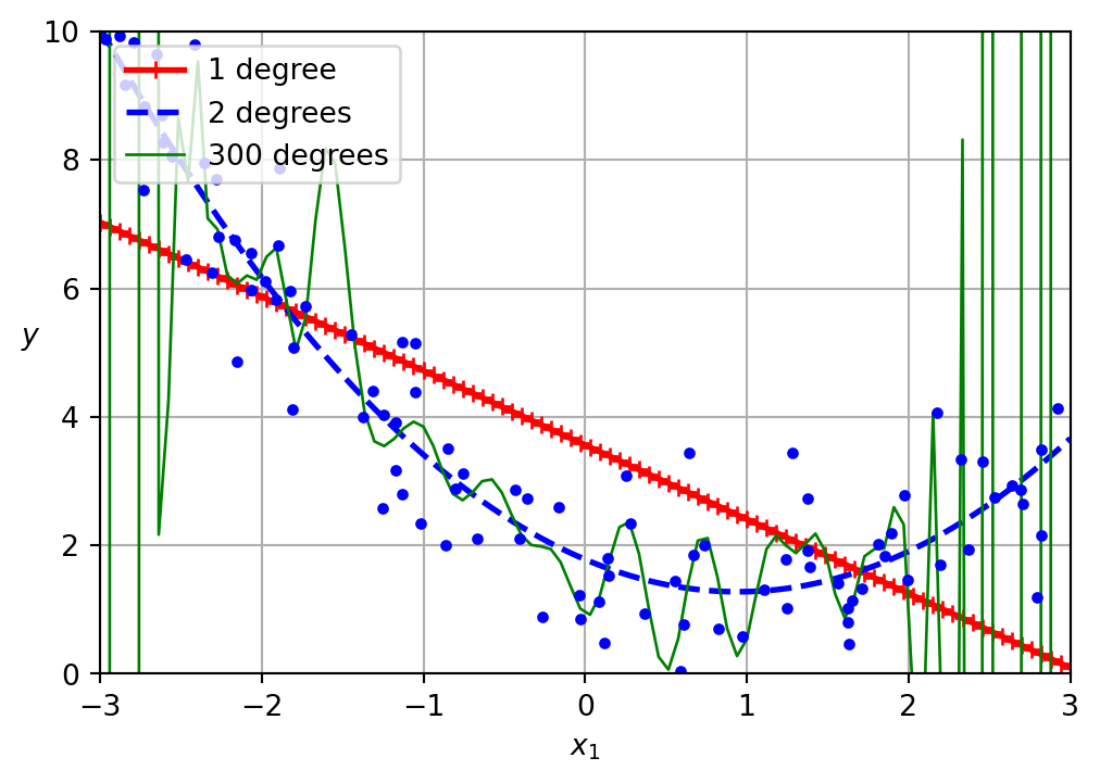
A linear model inadequately represents this dataset

Definition

Feature engineering is the process of creating, transforming, and selecting variables (attributes) from raw data to improve the performance of machine learning models.

Here, our focus is on creating new attributes from raw data.

PolynomialFeatures

from sklearn.preprocessing import PolynomialFeatures

poly_features = PolynomialFeatures(degree=2, include_bias=False)
X_poly = poly_features.fit_transform(X)

X[0]

array([-0.75275929])

X_poly[0]

array([-0.75275929,  0.56664654])

sklearn.preprocessing.PolynomialFeatures

Generate a new feature matrix consisting of all polynomial combinations of the features with degree less than or equal to the specified degree. For example, if an input sample is two dimensional and of the form \([a, b]\), the degree-2 polynomial features are \([1, a, b, a^2, ab, b^2]\).

PolynomialFeatures

Given two features \(a\) and \(b\), PolynomialFeatures with degree=3 would add \(a^2\), \(a^3\), \(b^2\), \(b^3\), as well as, \(ab\), \(a^2b\), \(ab^2\)!

Warning

PolynomialFeatures(degree=d) adds \(\frac{(D+d)!}{d!D!}\) features, where \(D\) is the original number of features.

Additionally, you have the option to engineer new features of your own.

Polynomial regression

LinearRegression on PolynomialFeatures

lin_reg = LinearRegression()
lin_reg.fit(X_poly, y)

Polynomial regression

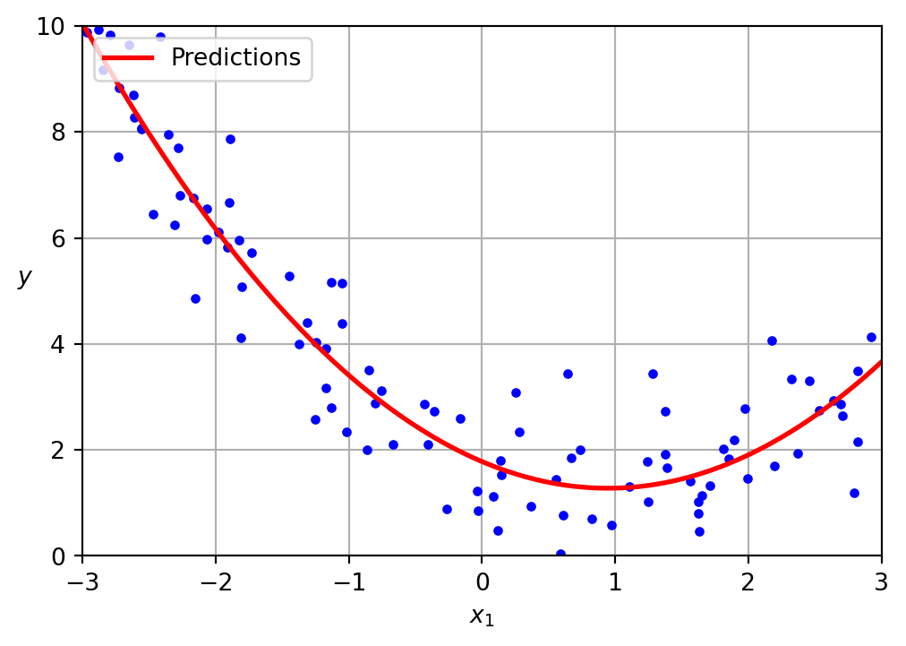
The data was generated according to the following equation, with the inclusion of Gaussian noise.

\[ y = 0.5 x^2 + 1.0 x + 2.0 \]

Presented below is the learned model.

\[ \hat{y} = 0.56 x^2 + (-1.06) x + 1.78 \]

lin_reg.coef_, lin_reg.intercept_

(array([[-1.06633107,  0.56456263]]), array([1.78134581]))

Given the noise present in our dataset, akin to what we would expect with real-world data, this model demonstrates a good fit.

Overfitting and underfitting

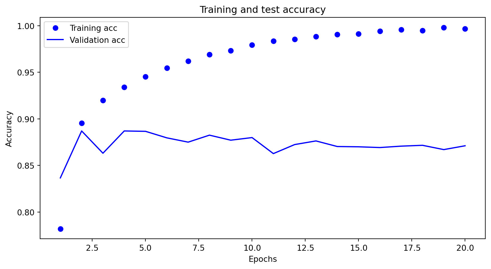
A low loss value on the training set does not necessarily indicate a “better” model.

In this example, the linear regression model is underfitting the training data, as indicated by its high mean squared error (loss) on the training set (red line). This suggests that the model makes numerous errors even on the training data.

Conversely, the polynomial model with degree=300 is overfitting the training data. It exhibits a low mean squared error (loss) on the training set (green line), implying that it makes few errors on the training data.

However, the degree=300 polynomial model is likely to perform poorly on future predictions. The green curve extends beyond the boundaries of the image on the y-axis. For instance, for input values in the range of 2 to 3, the model predicts values exceeding 10 (as well as negative values), whereas the expected values should lie within the range of 2 to 4.

This illustrative example may seem simplistic since the data is generated from a quadratic equation and involves only a single attribute, making visualization straightforward. However, it serves to highlight a key point relevant to more complex models, such as deep neural networks. As the number of parameters increases, the model’s capacity to fit the training data also increases, which can lead to overfitting if not properly managed.

Attribution: 04_training_linear_models.ipynb

Under- and over- fitting

• Underfitting:
  • Your model is too simple (here, linear).
  • Uninformative features.
  • Poor performance on both training and test data.
• Overfitting:
  • Your model is too complex (tall decision tree, deep and wide neural networks, etc.).
  • Too many features given the number of examples available.
  • Excellent performance on the training set, but poor performance on the test set.

In the case of underfitting, adding more data to the training set will not help.

In the case of overfitting, adding more data would bring the train and test set learning curves closer.

Learning curves

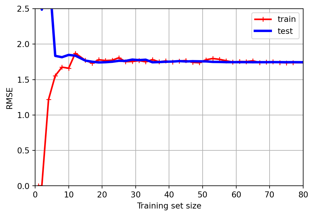
• One way to assess our models is to visualize the learning curves:
  • A learning curve shows the performance of our model, here using RMSE, on both the training set and the test set.
  • Multiple measurements are obtained by repeatedly training the model on larger and larger subsets of the data.

See: sklearn.model_selection.learning_curve.

Learning curve – underfitting

Poor performance on both training and test data.

This graph illustrates the learning curve for a linear regression model applied to data generated from a quadratic equation, which serves as our ongoing example.

The horizontal axis represents the size of the training set. Initially, the linear regression model is trained on a very small dataset, consisting of just one or a few examples, and the Root Mean Square Error (RMSE) is plotted for both the training and test sets. The size of the training set is then incrementally increased, a new model is trained, and the performance is recorded. This procedure continues until the entire dataset is utilized.

Key observations from the graph include:

• With only one or two examples, the model perfectly fits the training set, resulting in low RMSE for the training data.

• As the size of the training set increases, the model struggles to fit the training data due to the quadratic nature of the data generation process. Consequently, the RMSE for the training set rises and stabilizes at a higher level.

• For small training sets, the model performs poorly on the test set due to inadequate generalization, resulting in high RMSE.

• As the training set size grows, the test set performance improves, indicated by decreasing RMSE, until it reaches a point where further increases in training set size do not yield significant improvements.

These learning curves are indicative of a model that is underfitting. Both the training and test set RMSE curves plateau at relatively high values and remain close to each other, as noted by Géron (2022).

Source code: 04_training_linear_models.ipynb.

Learning curve – overfitting

Excellent performance on the training set, but poor performance on the test set.

• For a training set of up to 14 data points, the polynomial fits the training data perfectly, resulting in an RMSE of zero.

• The error on the training data in this instance is significantly lower.

• A notable gap between the two curves indicates that the model performs substantially better on the training data compared to the test data.

Polynomial with degree=14.

Overfitting - deep nets - loss

Neural networks will be covered in detail later in our course. The graph presented here illustrates the variation in the loss function as a deep learning model undergoes training.

This example utilizes the IMDB movie review sentiment classification dataset available in Keras. The dataset comprises 25,000 movie reviews from IMDB, each labeled with a sentiment (positive or negative).

The model consists of three dense layers with sizes 16, 16, and 1, respectively. It includes a total of 160,305 trainable parameters.

The network is trained using mini-batch stochastic gradient descent with a batch size of 512. The horizontal axis represents the number of epochs, where each epoch indicates that the model has seen the entire training set once. During each epoch, the stochastic gradient descent algorithm updates the model parameters iteratively using mini-batches of 512 examples.

I selected this example to illustrate that a neural network with with sufficient capacity (number of parameters) can minimize training errors almost to zero, as reducing training error is the primary objective of optimization. However, the graph clearly demonstrates that beyond a certain point, the learned patterns become specific to the training set rather than general principles. Generalization, rather than mere memorization, is the ultimate goal of machine learning.

Overfitting occurs when a model learns the details and noise in the training data to an extent that it negatively impacts the model’s performance on new data. This can result in a decision boundary that fits the training data too tightly, capturing noise and irrelevant details rather than general patterns.

Example from Chollet (2017) Chapter 3 (chapter04_getting-started-with-neural-networks.ipynb, ipynb from 2021 edition).

Overfitting - deep nets - accuracy

This graph similarly illustrates the variation in accuracy for both the training and test sets as the model undergoes training.

Bias/Variance Tradeoff

• Bias:
  • Error from overly simplistic models
  • High bias can lead to underfitting
• Variance:
  • Error from overly complex models
  • Sensitivity to fluctuations in the training data
  • High variance can lead to overfitting
• Tradeoff:
  • Aim for a model that generalizes well to new data
  • Methods: cross-validation, regularization, ensemble learning

Hastie, Tibshirani, and Friedman (2009)

Related videos

Other videos include:

• Bias and Variance, StatQuest (great visual summary)
• Bias/Variance (C2W1L02), Stanford, Andrew Ng
• Intuition behind bias and variance, Sebastian Raschka

Performance metrics

Confusion matrix

	Positive (Predicted)	Negative (Predicted)
Positive (Actual)	True positive (TP)	False negative (FN)
Negative (Actual)	False positive (FP)	True negative (TN)

• In statistical analysis, False Positives (FP) are commonly referred to as Type I errors, and False Negatives (FN) are known as Type II errors.

• The confusion matrix encapsulates all essential information required to assess the performance of a classification model.

• While the confusion matrix provides a comprehensive view, more concise metrics such as accuracy, precision, recall, and the F\(_1\) score are often more intuitive and practical for summarizing model performance.

A confusion matrix is a table summarizing the performance of a classification algorithm (here for a binary classification task).

sklearn.metrics.confusion_matrix

from sklearn.metrics import confusion_matrix

y_actual = [0, 0, 0, 1, 1, 1, 1, 1, 1, 1]
y_pred   = [0, 1, 1, 0, 0, 0, 1, 1, 1, 1]

confusion_matrix(y_actual,y_pred)

array([[1, 2],
       [3, 4]])

tn, fp, fn, tp = confusion_matrix(y_actual, y_pred).ravel()
(tn, fp, fn, tp)

(1, 2, 3, 4)

Perfect prediction

y_actual = [0, 1, 0, 0, 1, 1, 1, 0, 1, 1]
y_pred   = [0, 1, 0, 0, 1, 1, 1, 0, 1, 1]

confusion_matrix(y_actual,y_pred)

array([[4, 0],
       [0, 6]])

tn, fp, fn, tp = confusion_matrix(y_actual, y_pred).ravel()    
(tn, fp, fn, tp)

(4, 0, 0, 6)

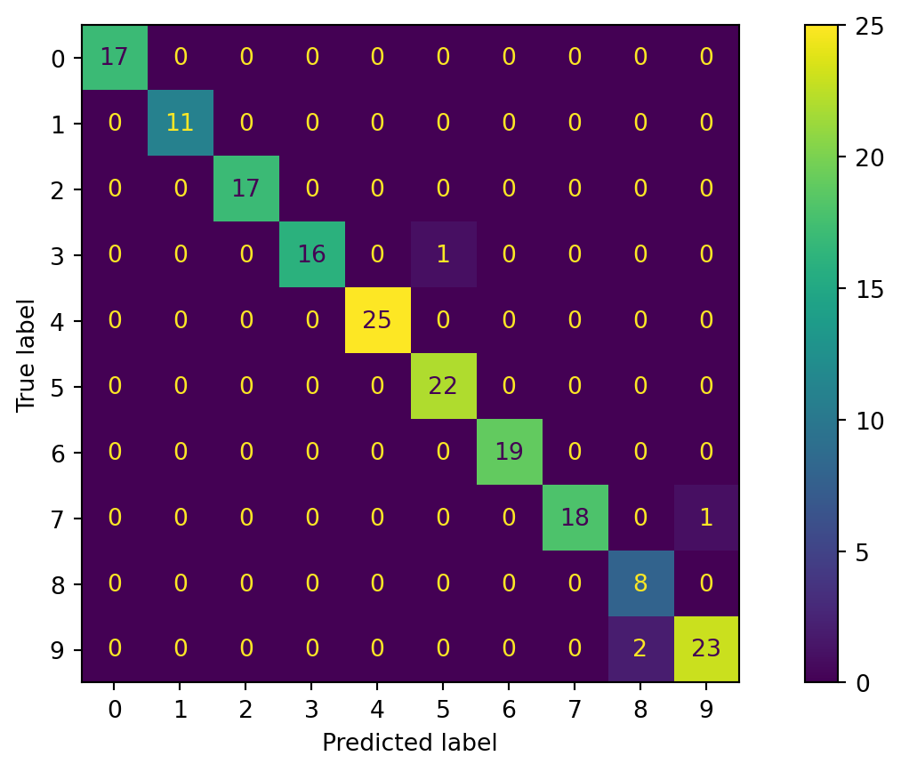
Confusion matrix - multiple classes

The image displays a heatmap of the confusion matrix for the digit classification task. This task, a multiclass classification problem, was addressed using OneVsRestClassifier and LogisticRegression.

The confusion matrix summarizes the predictions made on the test set, which is a subset of the data that was neither used for training nor for preprocessing with StandardScaler.

The confusion matrix encapsulates all the results from applying the classifier to the test set. However, to summarize this information more succinctly, we often refer to performance metrics.

Confusion matrix for the digits example presented in the previous lecture.

Source code

import numpy as np
np.random.seed(42)

from sklearn.datasets import load_digits
digits = load_digits()

X = digits.data
y = digits.target

from sklearn.model_selection import train_test_split

X_train, X_test, y_train, y_test = train_test_split(X, y, test_size=0.1)

from sklearn.preprocessing import StandardScaler

scaler = StandardScaler()
X_train = scaler.fit_transform(X_train)

from sklearn.linear_model import LogisticRegression
from sklearn.multiclass import OneVsRestClassifier

clf = OneVsRestClassifier(LogisticRegression())

clf = clf.fit(X_train, y_train)

import matplotlib.pyplot as plt
from sklearn.metrics import ConfusionMatrixDisplay

X_test = scaler.transform(X_test)
y_pred = clf.predict(X_test)

ConfusionMatrixDisplay.from_predictions(y_test, y_pred)

plt.show()

Visualizing errors

mask = (y_test == 9) & (y_pred == 8)

X_9_as_8 = X_test[mask]

y_9_as_8 = y_test[mask]

In the confusion matrix on the previous screen, we had seen that there were examples for which the true label was 9, but the prediction was was 8. We can visualize the examples to see if we understand the nature of those errors.

Confusion matrix - multiple classes

It is often preferable to summarize the classifier’s performance with a single metric.

Accuracy

How accurate is this result?

\[ \mathrm{accuracy} = \frac{\mathrm{TP}+\mathrm{TN}}{\mathrm{TP}+\mathrm{TN}+\mathrm{FP}+\mathrm{FN}} = \frac{\mathrm{TP}+\mathrm{TN}}{\mathrm{N}} \]

from sklearn.metrics import accuracy_score

y_actual = [0, 0, 0, 1, 1, 1, 1, 1, 1, 1]
y_pred   = [0, 1, 1, 0, 0, 0, 1, 1, 1, 1]

accuracy_score(y_actual,y_pred)

0.5

Accuracy is the ratio of correctly predicted instances to the total number of predictions.

Accuracy

y_actual = [0, 1, 0, 0, 1, 1, 1, 0, 1, 1]
y_pred   = [1, 0, 1, 1, 0, 0, 0, 1, 0, 0]

accuracy_score(y_actual,y_pred)

0.0

y_actual = [0, 1, 0, 0, 1, 1, 1, 0, 1, 1]
y_pred   = [0, 1, 0, 0, 1, 1, 1, 0, 1, 1]

accuracy_score(y_actual,y_pred)

1.0

Accuracy is a number between 0 (all wrong) and 1 (perfect).

Accuracy can be misleading

y_actual = [0, 0, 0, 0, 1, 1, 0, 0, 0, 0]
y_pred   = [0, 0, 0, 0, 0, 0, 0, 0, 0, 0]

accuracy_score(y_actual,y_pred)

0.8

Accuracy can be misleading in the context of class imbalance, as it disproportionately reflects the performance on the majority class, thereby masking poor performance on the minority class.

As class imbalance increases, the accuracy metric becomes increasingly misleading.

Why is it problematic?

Precision

AKA, positive predictive value (PPV).

\[ \mathrm{precision} = \frac{\mathrm{TP}}{\mathrm{TP}+\mathrm{FP}} \]

from sklearn.metrics import precision_score

y_actual = [0, 0, 0, 1, 1, 1, 1, 1, 1, 1]
y_pred   = [0, 1, 1, 0, 0, 0, 1, 1, 1, 1]

precision_score(y_actual, y_pred)

0.6666666666666666

Precision is the proportion of true positive predictions among all positive predictions.

Precision alone is not enough

y_actual = [0, 0, 0, 1, 1, 1, 1, 1, 1, 1]
y_pred   = [0, 0, 0, 0, 0, 0, 1, 0, 0, 0]

precision_score(y_actual,y_pred)

1.0

An algorithm that makes a small number of high-confidence predictions might achieve a high precision score, but this may not necessarily be useful.

Recall

AKA sensitivity or true positive rate (TPR) \[ \mathrm{recall} = \frac{\mathrm{TP}}{\mathrm{TP}+\mathrm{FN}} \]

from sklearn.metrics import recall_score

y_actual = [0, 0, 0, 1, 1, 1, 1, 1, 1, 1]
y_pred   = [0, 1, 1, 0, 0, 0, 1, 1, 1, 1]

recall_score(y_actual,y_pred)

0.5714285714285714

Recall is the proportion of true positive instances correctly identified among all actual positive instances.

F\(_1\) score

\[ \begin{align*} F_1~\mathrm{score} &= \frac{2}{\frac{1}{\mathrm{precision}}+\frac{1}{\mathrm{recall}}} = 2 \times \frac{\mathrm{precision}\times\mathrm{recall}}{\mathrm{precision}+\mathrm{recall}} \\ &= \frac{\mathrm{TP}}{\mathrm{FP}+\frac{\mathrm{FN}+\mathrm{FP}}{2}} \end{align*} \]

from sklearn.metrics import f1_score

y_actual = [0, 0, 0, 1, 1, 1, 1, 1, 1, 1]
y_pred   = [0, 1, 1, 0, 0, 0, 1, 1, 1, 1]

f1_score(y_actual,y_pred)

0.6153846153846154

• The harmonic mean places greater emphasis on lower values, while the arithmetic mean treats all values equally.
• Using the harmonic mean ensures that a high score is only achieved when both precision and recall are high, thus providing a more holistic measure of a classifier’s performance in scenarios with imbalanced datasets.
• The F\(_1\) score favors classifiers that achieve a balance between precision and recall.
• Increasing recall often results in a decrease in precision, and vice versa. This phenomenon is known as the precision/recall trade-off.

F\(_1\) is the harmonic mean of precision and recall.

Micro Performance Metrics

Micro performance metrics aggregate the contributions of all classes to compute the average performance metric, such as precision, recall, or F1 score. This approach treats each individual prediction equally, providing a balanced evaluation by emphasizing the performance on frequent classes.

Macro Performance Metrics

Macro performance metrics compute the performance metric independently for each class and then average these metrics. This approach treats each class equally, regardless of its frequency, providing an evaluation that equally considers performance across both frequent and infrequent classes.

Micro/macro metrics

from sklearn.metrics import ConfusionMatrixDisplay

# Sample data
y_true = ['Cat'] * 42 + ['Dog'] *  7 + ['Fox'] * 11
y_pred = ['Cat'] * 39 + ['Dog'] *  1 + ['Fox'] *  2 + \
         ['Cat'] *  4 + ['Dog'] *  3 + ['Fox'] *  0 + \
         ['Cat'] *  5 + ['Dog'] *  1 + ['Fox'] *  5

ConfusionMatrixDisplay.from_predictions(y_true, y_pred)

The dataset can be conceptualized as resulting from an image classification task, involving images of cats, dogs, and foxes. Reflecting common trends observed on the internet, images of cats are disproportionately represented, leading to a class imbalance issue.

Micro/macro precision

from sklearn.metrics import classification_report, precision_score

print(classification_report(y_true, y_pred), "\n")

print("Micro precision: {:.2f}".format(precision_score(y_true, y_pred, average='micro')))
print("Macro precision: {:.2f}".format(precision_score(y_true, y_pred, average='macro')))

              precision    recall  f1-score   support

         Cat       0.81      0.93      0.87        42
         Dog       0.60      0.43      0.50         7
         Fox       0.71      0.45      0.56        11

    accuracy                           0.78        60
   macro avg       0.71      0.60      0.64        60
weighted avg       0.77      0.78      0.77        60
 

Micro precision: 0.78
Macro precision: 0.71

Macro-average precision is calculated as the mean of the precision scores for each class: \(\frac{0.81 + 0.60 + 0.71}{3} = 0.71\).

Whereas, the micro-average precision is calculated using the formala, \(\frac{TP}{TP+FP}\) and the data from the entire confusion matrix \(\frac{39+3+5}{39+3+5+9+2+2} = \frac{47}{60} = 0.78\)

The high micro-average precision observed here is primarily due to the high precision and large number of examples in the majority class, Cat. This masks the classifier’s relatively poor performance on the minority classes, Dog and Fox.

In a balanced dataset, both micro-average and macro-average metrics yield similar scores.

However, in an imbalanced dataset, significant disparities in classifier performance between the majority and minority classes will result in divergent micro-average and macro-average scores. Specifically, the classifier tends to underperform on the minority class(es), leading to these discrepancies.

In macro-average metrics, each class contributes equally to the final metric calculation, irrespective of the number of examples it contains. This means that the performance metric for each class are computed independently and then averaged, without considering the proportion of instances that each class represents in the dataset. Consequently, macro-averaging ensures that each class has an equal impact on the overall metric, which can be particularly useful in cases where the class distribution is imbalanced.

Micro/macro recall

              precision    recall  f1-score   support

         Cat       0.81      0.93      0.87        42
         Dog       0.60      0.43      0.50         7
         Fox       0.71      0.45      0.56        11

    accuracy                           0.78        60
   macro avg       0.71      0.60      0.64        60
weighted avg       0.77      0.78      0.77        60
 

Micro recall: 0.78
Macro recall: 0.60

Macro-average recall is calculated as the mean of the recall scores for each class: \(\frac{0.93 + 0.43 + 0.45}{3} = 0.60\).

Whereas, the micro-average recall is calculated using the formala, \(\frac{TP}{TP+FN}\) and the data from the entire confusion matrix \(\frac{39+3+5}{39+3+5+3+4+6} = \frac{39}{60} = 0.78\)

Micro/macro metrics (medical data)

Consider a medical dataset, such as those involving diagnostic tests or imaging, comprising 990 normal samples and 10 abnormal (tumor) samples. This represents the ground truth.

Micro/macro metrics (medical data)

              precision    recall  f1-score   support

      Normal       1.00      0.99      1.00       990
      Tumour       0.55      0.60      0.57        10

    accuracy                           0.99      1000
   macro avg       0.77      0.80      0.78      1000
weighted avg       0.99      0.99      0.99      1000
 

Micro precision: 0.99
Macro precision: 0.77


Micro recall: 0.99
Macro recall: 0.80

Hand-written digits (revisited)

Loading the dataset

import numpy as np
np.random.seed(42)

from sklearn.datasets import fetch_openml

digits = fetch_openml('mnist_784', as_frame=False)
X, y = digits.data, digits.target

Plotting the first five examples

These images have dimensions of ( 28 ) pixels.

Creating a binary classification task

# Creating a binary classification task (one vs the rest)

some_digit = X[0]
some_digit_y = y[0]

y = (y == some_digit_y)
y

array([ True, False, False, ..., False,  True, False])

# Creating the training and test sets
from sklearn.model_selection import train_test_split

X_train, X_test, y_train, y_test = train_test_split(X, y, test_size=0.1)

SGDClassifier

from sklearn.linear_model import SGDClassifier

clf = SGDClassifier()
clf.fit(X_train, y_train)

clf.predict(X[0:5]) # small sanity check

array([ True, False, False, False, False])

The SGDClassifier is a linear classifier that utilizes stochastic gradient descent (SGD) for training. Compared to LogisticRegression, it can offer faster training times, particularly for large datasets. Additionally, SGDClassifier allows for the adjustment of the decision threshold in subsequent examples.

Performance

from sklearn.metrics import accuracy_score

y_pred = clf.predict(X_test)

accuracy_score(y_test, y_pred)

0.9572857142857143

Wow!

Not so fast

y_pred = dummy_clf.predict(X_test)

accuracy_score(y_test, y_pred)

0.906

Why is the accuracy so high despite this classifier ignoring the input data?

The high accuracy is attributed to the class distribution within the dataset. Approximately 10% of the samples correspond to the digit ‘5’, which is the positive class in our binary classification task. Consequently, about 90% of the samples are ‘not 5’ and belong to the negative class. Since the DummyClassifier always predicts the majority class, its accuracy is expected to be around 90%.

This underscores the point that accuracy is often not the best metric, particularly when dealing with imbalanced datasets.

The DummyClassifier in scikit-learn generates predictions without considering the input features. By default, it consistently predicts the most frequent class label in the training data. It is a simple baseline classifier.

Precision-recall trade-off

Attribution: Géron (2022) Figure 3.4

Precision-recall trade-off

As the decision threshold decreases, a higher number of examples are predicted as positive, potentially leading the classifier to eventually label all instances as positive.

Conversely, as the decision threshold increases, fewer examples are classified as positive, which may result in the classifier predicting no positive instances at all.

For certain applications, a classifier with high precision is essential. For example, consider a scenario where each prediction necessitates a costly laboratory experiment to verify its accuracy, such as in a pharmaceutical company aiming to discover new drugs. Here, the classifier predicts whether a compound is active. Given the high cost of experiments to validate candidates, the company would prioritize focusing on the most promising compounds first.

In contrast, consider a scenario involving cancer screening, such as using mammograms to detect breast cancer. In this case, it may be preferable to lower the decision threshold, thereby increasing the number of false-positive predictions. Although this approach results in more patients undergoing additional tests, such as biopsies, it can potentially save more lives by ensuring that fewer cases of cancer go undetected.

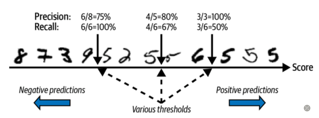
I have used SGDClassifier because it allows to vary the decision treshold (boundary) to produce a plot illustrating the precision-recall tradeoff.

Precision/Recall curve

ROC curve

Receiver Operating Characteristics (ROC) curve

• True positive rate (TPR) against false positive rate (FPR)
• An ideal classifier has TPR close to 1.0 and FPR close to 0.0
• \(\mathrm{TPR} = \frac{\mathrm{TP}}{\mathrm{TP}+\mathrm{FN}}\) (recall, sensitivity)
• TPR approaches one when the number of false negative predictions is low
• \(\mathrm{FPR} = \frac{\mathrm{FP}}{\mathrm{FP}+\mathrm{TN}}\) (aka~[1-specificity])
• FPR approaches zero when the number of false positive is low

ROC (Receiver Operating Characteristic) curves are popular in machine learning and statistics for several reasons:

1. Comprehensive Performance Evaluation: ROC curves provide a visual representation of a classifier’s performance across all possible thresholds. By plotting the True Positive Rate (TPR) against the False Positive Rate (FPR), it allows practitioners to evaluate the trade-off between sensitivity (recall) and specificity.
2. Threshold Independence: Unlike metrics like accuracy, ROC curves evaluate classifier performance without relying on a specific decision threshold. This makes them particularly useful in comparing models across varying thresholds.
3. Handling Imbalanced Datasets: For datasets with class imbalances (where one class is much more frequent than the other), ROC curves are more informative than accuracy, which can be misleading. The curve captures the model’s ability to distinguish between classes irrespective of their distribution.
4. Area Under the Curve (AUC): The Area Under the ROC Curve (AUC) provides a single value summary of the model’s performance. AUC-ROC is often used as a benchmark metric to compare different models, with values ranging from 0.5 (random guessing) to 1.0 (perfect classification).
5. Broad Applicability: ROC curves can be used for any binary classification task and are easily extended to multiclass problems using techniques like one-vs-rest classification, making them versatile in evaluating classifiers.

Overall, their ability to offer a broad, threshold-independent view of model performance, especially in imbalanced scenarios, makes ROC curves a popular choice for evaluating classifiers.

ROC curve

It is common to measure the area under the curve, represented as AUC. Specifically, the area under the ROC curve. This allows to compare

Attribution: 03_classification.ipynb

AUC/ROC

ROC curves provide a visual representation of a classifier’s performance across all possible thresholds. By plotting the True Positive Rate (TPR) against the False Positive Rate (FPR), it allows practitioners to evaluate the trade-off between sensitivity (recall) and specificity.

Unlike metrics like accuracy, ROC curves evaluate classifier performance without relying on a specific decision threshold. This makes them particularly useful in comparing models across varying thresholds.

The model was trained using the Pima Indians Diabetes dataset as described in Knowler et al. (1981) [PubMed]. Further details about the dataset will be discussed in the next lecture.

The 7 steps of machine learning

Prologue

Further reading

This book, which examines various aspects of the evaluation process with an emphasis on classification algorithms, has excellent ratings on Amazon!

Nathalie Japkowicz was formely a professor that the University of Ottawa. She now works at the American University in Washington.

Mohak Shah completed his PhD at the University of Ottawa. He has held several positions in the industry, including AI and Machine Learning Vice President for LG Electronics.

Japkowicz and Shah (2011)

Next lecture

• We will examine cross-validation and hyperparameter tuning.

References

Chollet, François. 2017. Deep Learning with Python. Manning Publications.

Géron, Aurélien. 2022. Hands-on Machine Learning with Scikit-Learn, Keras, and TensorFlow. 3rd ed. O’Reilly Media, Inc.

Hastie, Trevor, Robert Tibshirani, and Jerome H. Friedman. 2009. The Elements of Statistical Learning: Data Mining, Inference, and Prediction, 2nd Edition. Springer Series in Statistics. Springer. https://doi.org/10.1007/978-0-387-84858-7.

Japkowicz, Nathalie, and Mohak Shah. 2011. Evaluating Learning Algorithms: A Classification Perspective. Cambridge: Cambridge University Press. http://assets.cambridge.org/97805211/96000/cover/9780521196000.jpg.

Knowler, William C., David J. Pettitt, Peter J. Savage, and Peter H. Bennett. 1981. “Diabetes Incidence in Pima Indians: Contributions of Obesity and Parental Diabetes.” American Journal of Epidemiology 113 2: 144–56. https://api.semanticscholar.org/CorpusID:25209675.

Russell, Stuart, and Peter Norvig. 2020. Artificial Intelligence: A Modern Approach. 4th ed. Pearson. http://aima.cs.berkeley.edu/.

Marcel Turcotte

[email protected]

School of Electrical Engineering and Computer Science (EECS)

University of Ottawa