Local Search
CSI 4106 - Fall 2024
Version: Nov 17, 2024 09:21
Preamble
Quote of the Day
Learning Objectives
- Understand the concept and application of local search algorithms in optimization problems.
- Implement and analyze the hill-climbing algorithm, recognizing its limitations such as local maxima and plateaus.
- Apply effective state representation strategies in problems like the 8-Queens to enhance search efficiency.
- Explain how simulated annealing overcomes local optima by allowing probabilistic acceptance of worse states.
- Analyze the influence of temperature and energy difference on the acceptance probability in simulated annealing.
- Recognize the application of simulated annealing in solving complex optimization problems like the Travelling Salesman Problem (TSP).
Introduction
Context
Focus has been on finding paths in state space.
Some problems prioritize the goal state over the path.
- Integrated-circuit design
- Job shop scheduling
- Automatic programming
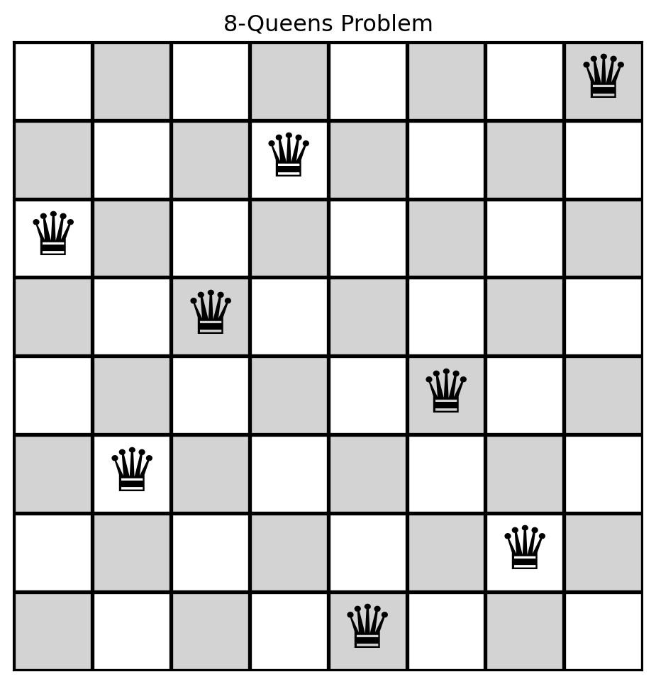
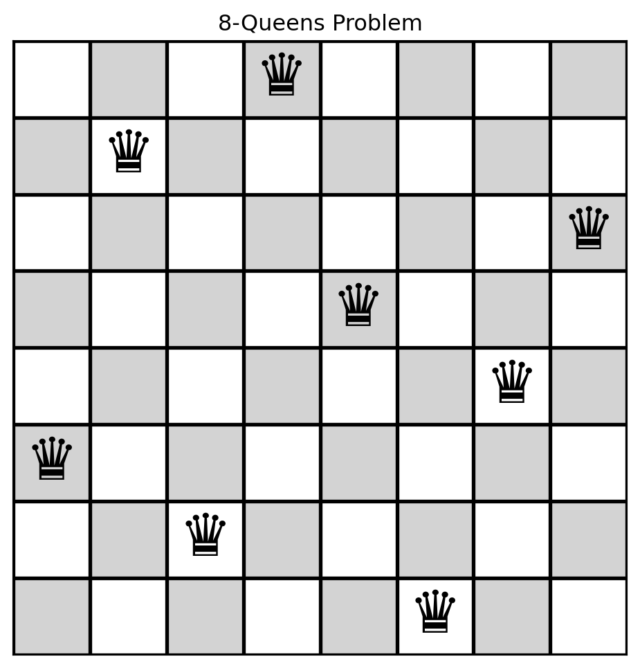
8-Queens Problem
Definition
Local search algorithms operate by searching from a start state to neighboring states, without keeping track of the paths, nor the set of states that have been reached.
Problem Definition
Find the “best” state according to an objective function, thereby locating the global maximum.
Hill-Climbing
Hill-Climbing
Hill-Climbing
Given as in input a problem
current is the initial state of problem
while not done do
- nighbour is the highest-valued successor state of current
- if value(neighbour) \(\le\) value(current) the return current
- set current to neighbour
8-Queens
How would you represent the current state?
Why is using a grid to represent the current state suboptimal?
A grid representation permits the illegal placement of two queens in the same column.
Instead, we can represent the state as a list (\(\mathrm{state}\)), where each element corresponds to the row position of the queen in its respective column.
In other words, \(\mathrm{state}[i]\) is the row of the queen is column \(i\).
State Representation
create_initial_state
create_initial_state
Representation of 8-Queens
\(8 \times 8\) chessboard.
Unconstrained Placement: \(\binom{64}{8} = 4,426,165,368\) possible configurations, representing the selection of 8 squares from 64.
Column Constraint: Use a list of length 8, with each entry indicating the row of a queen in its respective column, resulting in \(8^8 = 16,777,216\) configurations.
Row and Column Constraints: Model board states as permutations of the 8 row indices, reducing configurations to \(8! = 40,320\).
create_initial_state
create_initial_state
calculate_conflicts
def calculate_conflicts(state):

    n = len(state)
    conflicts = 0

    for col_i in range(n):
        for col_j in range(col_i + 1, n):
            row_i = state[col_i]
            row_j = state[col_j]
            if row_i == row_j:                 # same row
                conflicts += 1
            if col_i - row_i == col_j - row_j: # same diagonal
                conflicts += 1
            if col_i + row_i == col_j + row_j: # same anti-diagonal
                conflicts += 1

    return conflicts
calculate_conflicts
get_neighbors_rn
def get_neighbors_rn(state):

    """Generates neighboring states by moving on queen at a time to a new row."""

    neighbors = []
    n = len(state)

    for col in range(n):
        for row in range(n):
            if (state[col] != row):
              new_state = state[:] # create a copy of the state
              new_state[col] = row
              neighbors.append(new_state)

return neighborsget_neighbors_rn
initial_state_8 = create_initial_state(8)
print(initial_state_8)
for s in get_neighbors_rn(initial_state_8):
  print(f"{s} -> # of conflicts = {calculate_conflicts(s)}")
[3, 2, 7, 1, 6, 0, 4, 5]
[0, 2, 7, 1, 6, 0, 4, 5] -> # of conflicts = 5
[1, 2, 7, 1, 6, 0, 4, 5] -> # of conflicts = 6
[2, 2, 7, 1, 6, 0, 4, 5] -> # of conflicts = 6
[4, 2, 7, 1, 6, 0, 4, 5] -> # of conflicts = 6
[5, 2, 7, 1, 6, 0, 4, 5] -> # of conflicts = 7
[6, 2, 7, 1, 6, 0, 4, 5] -> # of conflicts = 5
[7, 2, 7, 1, 6, 0, 4, 5] -> # of conflicts = 5
[3, 0, 7, 1, 6, 0, 4, 5] -> # of conflicts = 5
[3, 1, 7, 1, 6, 0, 4, 5] -> # of conflicts = 5
[3, 3, 7, 1, 6, 0, 4, 5] -> # of conflicts = 7
[3, 4, 7, 1, 6, 0, 4, 5] -> # of conflicts = 7
[3, 5, 7, 1, 6, 0, 4, 5] -> # of conflicts = 5
[3, 6, 7, 1, 6, 0, 4, 5] -> # of conflicts = 6
[3, 7, 7, 1, 6, 0, 4, 5] -> # of conflicts = 5
[3, 2, 0, 1, 6, 0, 4, 5] -> # of conflicts = 9
[3, 2, 1, 1, 6, 0, 4, 5] -> # of conflicts = 8
[3, 2, 2, 1, 6, 0, 4, 5] -> # of conflicts = 7
[3, 2, 3, 1, 6, 0, 4, 5] -> # of conflicts = 8
[3, 2, 4, 1, 6, 0, 4, 5] -> # of conflicts = 7
[3, 2, 5, 1, 6, 0, 4, 5] -> # of conflicts = 7
[3, 2, 6, 1, 6, 0, 4, 5] -> # of conflicts = 6
[3, 2, 7, 0, 6, 0, 4, 5] -> # of conflicts = 6
[3, 2, 7, 2, 6, 0, 4, 5] -> # of conflicts = 5
[3, 2, 7, 3, 6, 0, 4, 5] -> # of conflicts = 4
[3, 2, 7, 4, 6, 0, 4, 5] -> # of conflicts = 5
[3, 2, 7, 5, 6, 0, 4, 5] -> # of conflicts = 5
[3, 2, 7, 6, 6, 0, 4, 5] -> # of conflicts = 6
[3, 2, 7, 7, 6, 0, 4, 5] -> # of conflicts = 6
[3, 2, 7, 1, 0, 0, 4, 5] -> # of conflicts = 6
[3, 2, 7, 1, 1, 0, 4, 5] -> # of conflicts = 6
[3, 2, 7, 1, 2, 0, 4, 5] -> # of conflicts = 8
[3, 2, 7, 1, 3, 0, 4, 5] -> # of conflicts = 5
[3, 2, 7, 1, 4, 0, 4, 5] -> # of conflicts = 5
[3, 2, 7, 1, 5, 0, 4, 5] -> # of conflicts = 7
[3, 2, 7, 1, 7, 0, 4, 5] -> # of conflicts = 6
[3, 2, 7, 1, 6, 1, 4, 5] -> # of conflicts = 6
[3, 2, 7, 1, 6, 2, 4, 5] -> # of conflicts = 6
[3, 2, 7, 1, 6, 3, 4, 5] -> # of conflicts = 9
[3, 2, 7, 1, 6, 4, 4, 5] -> # of conflicts = 7
[3, 2, 7, 1, 6, 5, 4, 5] -> # of conflicts = 8
[3, 2, 7, 1, 6, 6, 4, 5] -> # of conflicts = 7
[3, 2, 7, 1, 6, 7, 4, 5] -> # of conflicts = 8
[3, 2, 7, 1, 6, 0, 0, 5] -> # of conflicts = 3
[3, 2, 7, 1, 6, 0, 1, 5] -> # of conflicts = 4
[3, 2, 7, 1, 6, 0, 2, 5] -> # of conflicts = 3
[3, 2, 7, 1, 6, 0, 3, 5] -> # of conflicts = 4
[3, 2, 7, 1, 6, 0, 5, 5] -> # of conflicts = 3
[3, 2, 7, 1, 6, 0, 6, 5] -> # of conflicts = 4
[3, 2, 7, 1, 6, 0, 7, 5] -> # of conflicts = 4
[3, 2, 7, 1, 6, 0, 4, 0] -> # of conflicts = 4
[3, 2, 7, 1, 6, 0, 4, 1] -> # of conflicts = 4
[3, 2, 7, 1, 6, 0, 4, 2] -> # of conflicts = 6
[3, 2, 7, 1, 6, 0, 4, 3] -> # of conflicts = 6
[3, 2, 7, 1, 6, 0, 4, 4] -> # of conflicts = 4
[3, 2, 7, 1, 6, 0, 4, 6] -> # of conflicts = 4
[3, 2, 7, 1, 6, 0, 4, 7] -> # of conflicts = 4get_neighbors
get_neighbors
print(initial_state_8)
for s in get_neighbors(initial_state_8):
  print(f"{s} -> # of conflicts = {calculate_conflicts(s)}")
[3, 2, 7, 1, 6, 0, 4, 5]
[2, 3, 7, 1, 6, 0, 4, 5] -> # of conflicts = 8
[7, 2, 3, 1, 6, 0, 4, 5] -> # of conflicts = 6
[1, 2, 7, 3, 6, 0, 4, 5] -> # of conflicts = 3
[6, 2, 7, 1, 3, 0, 4, 5] -> # of conflicts = 3
[0, 2, 7, 1, 6, 3, 4, 5] -> # of conflicts = 7
[4, 2, 7, 1, 6, 0, 3, 5] -> # of conflicts = 3
[5, 2, 7, 1, 6, 0, 4, 3] -> # of conflicts = 6
[3, 7, 2, 1, 6, 0, 4, 5] -> # of conflicts = 5
[3, 1, 7, 2, 6, 0, 4, 5] -> # of conflicts = 3
[3, 6, 7, 1, 2, 0, 4, 5] -> # of conflicts = 7
[3, 0, 7, 1, 6, 2, 4, 5] -> # of conflicts = 4
[3, 4, 7, 1, 6, 0, 2, 5] -> # of conflicts = 3
[3, 5, 7, 1, 6, 0, 4, 2] -> # of conflicts = 4
[3, 2, 1, 7, 6, 0, 4, 5] -> # of conflicts = 7
[3, 2, 6, 1, 7, 0, 4, 5] -> # of conflicts = 5
[3, 2, 0, 1, 6, 7, 4, 5] -> # of conflicts = 10
[3, 2, 4, 1, 6, 0, 7, 5] -> # of conflicts = 4
[3, 2, 5, 1, 6, 0, 4, 7] -> # of conflicts = 4
[3, 2, 7, 6, 1, 0, 4, 5] -> # of conflicts = 5
[3, 2, 7, 0, 6, 1, 4, 5] -> # of conflicts = 5
[3, 2, 7, 4, 6, 0, 1, 5] -> # of conflicts = 4
[3, 2, 7, 5, 6, 0, 4, 1] -> # of conflicts = 4
[3, 2, 7, 1, 0, 6, 4, 5] -> # of conflicts = 6
[3, 2, 7, 1, 4, 0, 6, 5] -> # of conflicts = 4
[3, 2, 7, 1, 5, 0, 4, 6] -> # of conflicts = 4
[3, 2, 7, 1, 6, 4, 0, 5] -> # of conflicts = 3
[3, 2, 7, 1, 6, 5, 4, 0] -> # of conflicts = 5
[3, 2, 7, 1, 6, 0, 5, 4] -> # of conflicts = 2hill_climbing
def hill_climbing(current_state):

    current_conflicts = calculate_conflicts(current_state)

    while True:

        if current_conflicts == 0:
          return curent_state

        neighbors = get_neighbors(current_state)

        conflicts = [calculate_conflicts(neighbor) for neighbor in neighbors]

        if (min(conflicts)) > current_conflicts:
          return None # No improvement found, stuck at local minimum

        arg_best = np.argmin(conflicts)
        curent_state = neighbors[arg_best]
current_conflicts = conflicts[arg_best]hill_climbing (take 2)
MAX_SIDE_MOVES = 100

def hill_climbing(current_state):

    conflicts_current_state = calculate_conflicts(current_state)
    side_moves = 0

    while True:

        if conflicts_current_state == 0:
          return current_state

        neighbors = get_neighbors(current_state)

        conflicts = [calculate_conflicts(voisin) for voisin in neighbors]

        if (min(conflicts)) > conflicts_current_state:
          return None  # No improvement, local maxima

        if (min(conflicts)) == conflicts_current_state:
          side_moves += 1  # Plateau

        if side_moves > MAX_SIDE_MOVES:
          return None

        arg_best = np.argmin(conflicts)
        current_state = neighbors[arg_best]
        conflicts_current_state = conflicts[arg_best]
Solve
Solve (2)
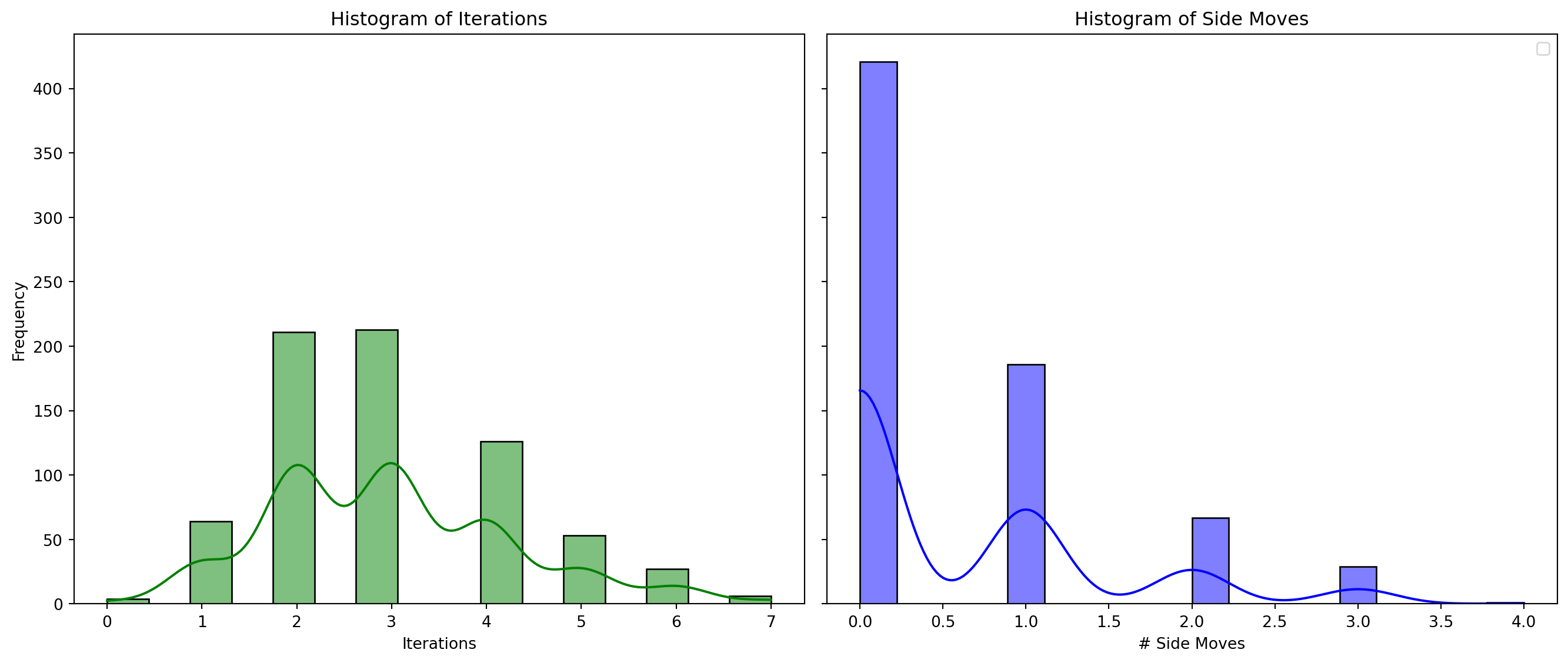
1000 runs, number of solutions = 704, 92 unique solutionsSolve 40-Queens
\(40! = 8.1591528325 \times 10^{47}\)
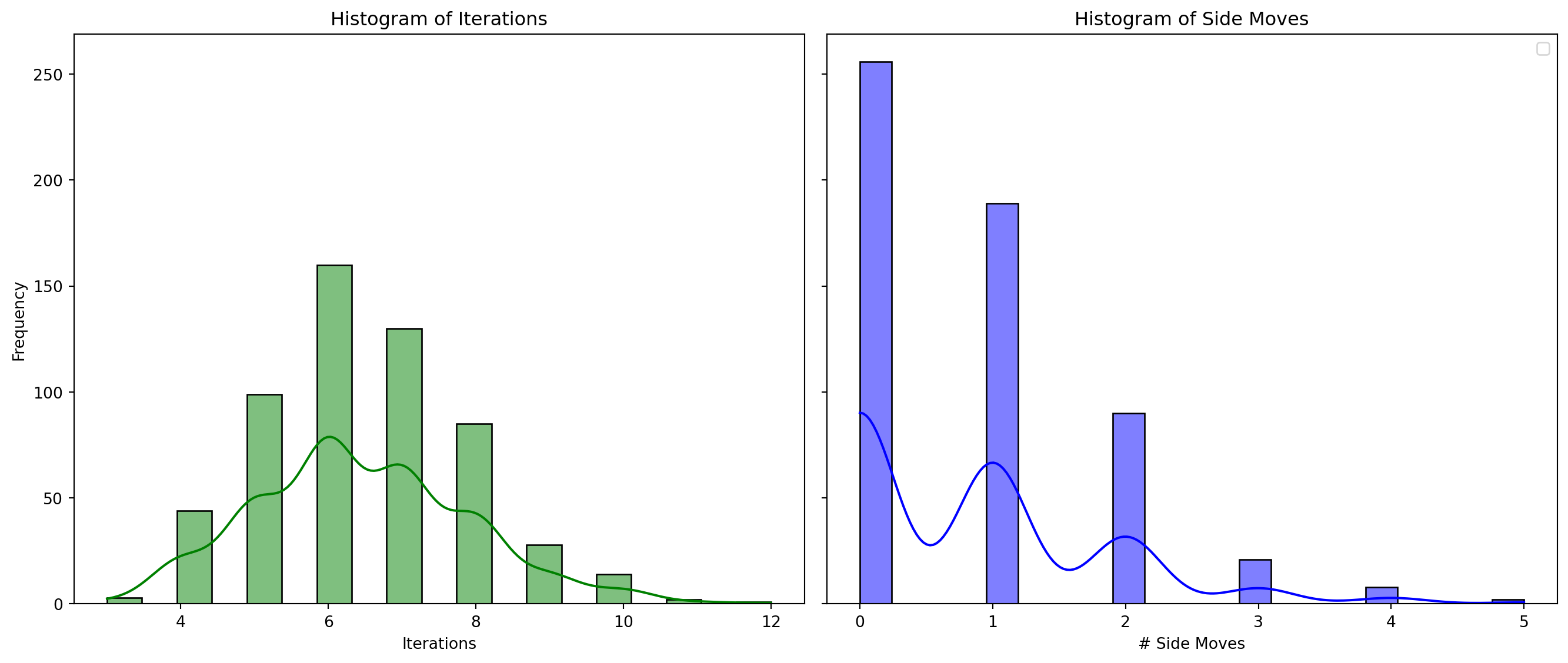
Iterations and Side Moves
1000 runs, number of solutions = 704, 92 unique solutions20-Queens
1000 runs, number of solutions = 566, 566 unique solutionsRussell & Norvig
- Hill climbing gets stuck 86% of the time.
- Successful attempts average 4 steps to a solution.
- Permitting 100 lateral moves boosts success rate from 14% to 94%.
- The problem space comprises \(8^8 = 16,777,216\) states.
- Implementation from Russell & Norvig
Escaping a Local Optimum
What mechanisms would enable the hill climbing algorithm to escape from a local optimum, whether it be a local minimum or maximum?
Remark
Assume the optimization problem is a minimization task, where the goal is to find a solution with the minimum cost.
Simulated Annealing
Definition
Simulated annealing is an optimization algorithm inspired by the annealing process in metallurgy. It probabilistically explores the solution space by allowing occasional uphill moves, which helps escape local optima. The algorithm gradually reduces the probability of accepting worse solutions by lowering a “temperature” parameter, ultimately converging towards an optimal or near-optimal solution.
Annealing
In metallurgy, annealing is the process used to temper or harden metals and glass by heating them to a high temperature and then gradually cooling them, thus allowing the material to reach a low-energy crystalline state.
Algorithm
Varying \(\Delta E\)
Varying the temperature, \(T\)
Varying the temperature and \(\Delta E\)
Varying the temperature and \(\Delta E\)
import { Inputs, Plot } from "@observablehq/plot"

viewof deltaE = Inputs.range([0.01, 100], {step: 0.01, value: 0.1, label: "ΔE", width: 300})

T_values = Array.from({length: 1000}, (_, i) => (i + 1) * 0.1)

function computeData(deltaE) {
  return T_values.map(T => ({
    T: T,
    value: Math.exp(-deltaE / T)
  }))
}

data = computeData(deltaE)

Plot.plot({
  marks: [
    Plot.line(data, {
      x: "T",
      y: "value",
      stroke: "steelblue",
      strokeWidth: 2
    }),
    Plot.ruleX([0], {stroke: "black"}), // X-axis line
    Plot.ruleY([0], {stroke: "black"})  // Y-axis line
  ]
})Theory
If the schedule lowers \(T\) to 0 slowly enough, then a property of the Boltzmann (aka Gibbs) distribution, \(e^{\frac{\Delta E}{T}}\), is that all the probability is concentrated on the global maxima, which the algorithm will find with probability approaching 1.
Definition
The Travelling Salesman Problem (TSP) is a classic optimization problem that seeks the shortest possible route for a salesman to visit a set of cities, returning to the origin city, while visiting each city exactly once.
How to Represent a Solution?
We will use a list where each element represents the index of a city, and the order of elements indicates the sequence of city visits.
Calculate the Total Distance
# Function to calculate the total distance of a given route

def calculate_total_distance(route, distance_matrix):

    total_distance = 0

    for i in range(len(route) - 1):
        total_distance += distance_matrix[route[i], route[i + 1]]

    total_distance += distance_matrix[route[-1], route[0]]  # Back to start

    return total_distance
Generating a Neighboring Solution
How to generate a neighboring solution?
Swap Two Cities
- Description: Select two cities at random and swap their positions.
- Pros: Simple and effective for exploring nearby solutions.
- Cons: Change may be too small, potentially slowing down convergence.
Reverse Segment
- Description: Select two indices and reverse the segment between them.
- Pros: More effective at finding shorter paths compared to simple swaps.
- Cons: Can still be computationally expensive as the number of cities increases.
Remove & Reconnect
- Description: Removes three edges from the route and reconnects the segments in the best possible way. This can generate up to 7 different routes.
- Pros: Provides more extensive changes and can escape local optima more effectively than 2-opt.
- Cons: More complex and computationally expensive to implement.
Insertion Move
- Description: Select a city and move it to a different position in the route.
- Pros: Offers a balance between small and large changes, making it useful for fine-tuning solutions.
- Cons: May require more iterations to converge to an optimal solution.
Shuffle Subset
- Description: Select a subset of cities in the route and randomly shuffle their order.
- Pros: Introduces larger changes and can help escape local minima.
- Cons: Can lead to less efficient routes if not handled carefully.
Generating a Neighboring Solution
simulated_annealing
def simulated_annealing(distance_matrix, initial_temp, cooling_rate, max_iterations):

    num_cities = len(distance_matrix)
    current_route = np.arange(num_cities)
    np.random.shuffle(current_route)
    current_cost = calculate_total_distance(current_route, distance_matrix)

    best_route = current_route.copy()
    best_cost = current_cost

    temperature = initial_temp

    for iteration in range(max_iterations):

        neighbor_route = get_neighbor(current_route)
        neighbor_cost = calculate_total_distance(neighbor_route, distance_matrix)

        # Accept the neighbor if it is better, or with a probability if it is worse.

        delta_E = neighbor_cost - current_cost

        if neighbor_cost < current_cost or np.random.rand() < np.exp(-(delta_E)/temperature):
            current_route = neighbor_route
            current_cost = neighbor_cost

            if current_cost < best_cost:
                best_route = current_route.copy()
                best_cost = current_cost

        # Cool down the temperature
        temperature *= cooling_rate

    return best_route, best_cost, temperatures, costs
Remarks
- As \(t \to \infty\), the algorithm exhibits behavior characteristic of a random walk. During this phase, any neighboring state, regardless of whether it improves the objective function, is accepted. This facilitates exploration and occurs at the start of the algorithm’s execution.
Remarks
- Conversely, as \(t \to 0\), the algorithm behaves like hill climbing. In this phase, only those states that enhance the objective function’s value are accepted, ensuring that the algorithm consistently moves towards optimal solutions—specifically, towards lower values in minimization problems. This phase emphasizes the exploitation of promising solutions and occurs towards the algorithm’s conclusion.
Example
# Ensuring reproducibility

np.random.seed(42)

# Generate random coordinates for cities

num_cities = 20
coordinates = np.random.rand(num_cities, 2) * 100

# Calculate distance matrix

distance_matrix = np.sqrt(((coordinates[:, np.newaxis] - coordinates[np.newaxis, :]) ** 2).sum(axis=2))

# Run simulated annealing

initial_temp = 15
cooling_rate = 0.995
max_iterations = 1000
Held–Karp Algorithm
- Introduced: 1962 by Held, Karp, and independently by Bellman.
- Problem: Solves the Traveling Salesman Problem (TSP) using dynamic programming.
- Time Complexity: \(\Theta(2^n n^2)\).
- Space Complexity: \(\Theta(2^n n)\).
- Efficiency: Better than brute-force \(\Theta(n!)\), yet still exponential.
Using Held–Karp to find the minimum cost of TSP tour: 386.43Execution
Best Route
Temperature and Cost
Swapping Neighbors
- Description: Select two cities at random, swap their positions.
- Pros: Simple and effective for exploring nearby solutions.
- Cons: Change may be too small, potentially slowing down convergence.
Execution
Best Route
Temperature and Cost
Selecting a Neighborhood Strategy
Simple Moves (Swap, Insertion): Effective for initial exploration; risk of local optima entrapment.
Complex Moves: Enhance capability to escape local optima and accelerate convergence; entail higher computational expense.
Hybrid Approaches: Integrate diverse strategies for neighborhood generation. Employ simple moves initially, transitioning to complex ones as convergence progresses.
Initial Temperature
Influence: Since the probability of accepting a new state is given by \(e^{-\frac{\Delta E}{T}}\), the selection of the initial temperature is directly influenced by \(\Delta E\) and consequently by the objective function value for a random state, \(f(s)\).
Initial Temperature
Example Problems: Consider two scenarios: problem \(a\) with \(f(a) = 1,000\) and problem \(b\) with \(f(b) = 100\).
Energy Difference: Accepting a state that is 10% worse results in energy differences \(\Delta E = 0.1 \cdot f(a) = 100\) for problem \(a\) and \(\Delta E = 0.1 \cdot f(b) = 10\) for problem \(b\).
Acceptance Probability: To accept such state 60% of the time, set \(e^{-\frac{\Delta E}{T}} = 0.6\). Solving for \(T\) yields initial temperatures of approximately \(T \approx 195.8\) for problem \(a\) and \(T \approx 19.58\) for problem \(b\).
Initial Temperature
A popular approach is to set the initial temperature so that a significant portion of moves (often around 60-80%) are accepted.
This can be done by running a preliminary phase where the temperature is adjusted until the acceptance ratio stabilizes within this range.
Cooling Strategies
In simulated annealing, cooling down is essential for managing algorithm convergence. The cooling schedule dictates the rate at which the temperature decreases, affecting the algorithm’s capacity to escape local optima and converge towards a near-optimal solution.
Linear Cooling
- Description: The temperature decreases linearly with each iteration.
- Formula: \(T = T_0 - \alpha \cdot k\)
- \(T_0\): Initial temperature
- \(\alpha\): A constant decrement
- \(k\): Current iteration
- Pros: Simple to implement and understand.
- Cons: Often leads to premature convergence because the temperature decreases too quickly.
Geometric (Exponential) Cooling
- Description: The temperature decreases exponentially with each iteration.
- Formula: \(T = T_0 \cdot \alpha^k\)
- \(\alpha\): Cooling rate, typically between 0.8 and 0.99
- \(k\): Current iteration
- Pros: Widely used due to its simplicity and effectiveness.
- Cons: The choice of \(\alpha\) is critical; if it’s too small, the temperature drops too fast, and if it’s too large, convergence can be slow.
Logarithmic Cooling
- Description: The temperature decreases slowly following a logarithmic function.
- Formula: \(T = \frac{\alpha \cdot T_0}{\log(1+k)}\)
- \(\alpha\): A scaling constant
- \(k\): Current iteration
- Pros: Provides a slower cooling rate, which is useful for problems that require extensive exploration of the solution space.
- Cons: Convergence can be very slow, requiring many iterations.
Inverse Cooling
- Description: The temperature decreases as an inverse function of the iteration number.
- Formula: \(T = \frac{T_0}{1+\alpha \cdot K}\)
- \(\alpha\): A scaling constant
- \(k\): Current iteration
- Pros: Allows for a more controlled cooling process, balancing exploration and exploitation.
- Cons: May require careful tuning of \(\alpha\) to be effective.
Adaptive Cooling
- Description: The cooling schedule is adjusted dynamically based on the performance of the algorithm.
- Strategy: If the algorithm is not making significant progress, the cooling rate may be slowed down. Conversely, if progress is steady, the cooling rate can be increased.
- Pros: More flexible and can adapt to the characteristics of the problem.
- Cons: More complex to implement and requires careful design to avoid instability.
Cooling Schedule - Summary
Choosing the Right Cooling Schedule
Problem-Specific: The choice of cooling schedule often depends on the characteristics of the problem being solved. Some problems benefit from a slower cooling rate, while others may need faster convergence.
Experimentation: It’s common to experiment with different strategies and parameters to find the best balance between exploration (searching broadly) and exploitation (refining the current best solutions).
Conclusion
After applying simulated annealing, a local search method such as hill climbing can be used to refine the solution.
Simulated annealing is effective for exploring the solution space and avoiding local minima, while local search focuses on the exploration of neighboring solutions.
Simulated Annealing Visualization
Prologue
Summary
- Local search algorithms focus on finding goal states by moving between neighboring states without tracking paths.
- The hill-climbing algorithm seeks the highest-valued neighbor but can get stuck in local maxima or plateaus.
- Effective state representation, such as using permutations in the 8-Queens problem, avoids illegal placements and improves performance.
- Simulated annealing allows occasional uphill moves to escape local optima, controlled by a decreasing temperature parameter.
- The acceptance probability in simulated annealing decreases as temperature lowers and energy difference increases.
- Simulated annealing effectively solves complex problems like the Travelling Salesman Problem by probabilistically exploring the solution space.
Further Readings
“The overall SA [simulated annealing] methodology is then deployed in detail on a real-life application: a large-scale aircraft trajectory planning problem involving nearly 30,000 flights at the European continental scale.”
Next lecture
- We will discuss population-based algorithms.
References
Marcel Turcotte
School of Electrical Engineering and Computer Science (EECS)
University of Ottawa


