import numpy as np

# Sample data

values = np.array([
    360, 83, 59, 130, 431, 67, 230, 52, 93, 125, 670, 892, 600, 38, 48, 147,
    78, 256, 63, 17, 120, 164, 432, 35, 92, 110, 22, 42, 50, 323, 514, 28,
    87, 73, 78, 15, 26, 78, 210, 36, 85, 189, 274, 43, 33, 10, 19, 389, 276,
    312])

weights = np.array([
    7, 0, 30, 22, 80, 94, 11, 81, 70, 64, 59, 18, 0, 36, 3, 8, 15, 42, 9, 0,
    42, 47, 52, 32, 26, 48, 55, 6, 29, 84, 2, 4, 18, 56, 7, 29, 93, 44, 71,
    3, 86, 66, 31, 65, 0, 79, 20, 65, 52, 13])

capacity = 850Population-Based Metaheuristics
CSI 4106 - Fall 2024
Version: Nov 17, 2024 11:46
Preamble
Quote of the Day
Learning Objectives
- Understand the definition and purpose of metaheuristics in optimization problems.
- Learn the principles and components of genetic algorithms (GAs).
- Comprehend the implementation details of GAs, including encoding, selection, crossover, mutation, and fitness evaluation.
- Apply GAs to solve the 0/1 knapsack problem with practical Python examples.
- Recognize different encoding schemes and selection methods in GAs.
Introduction
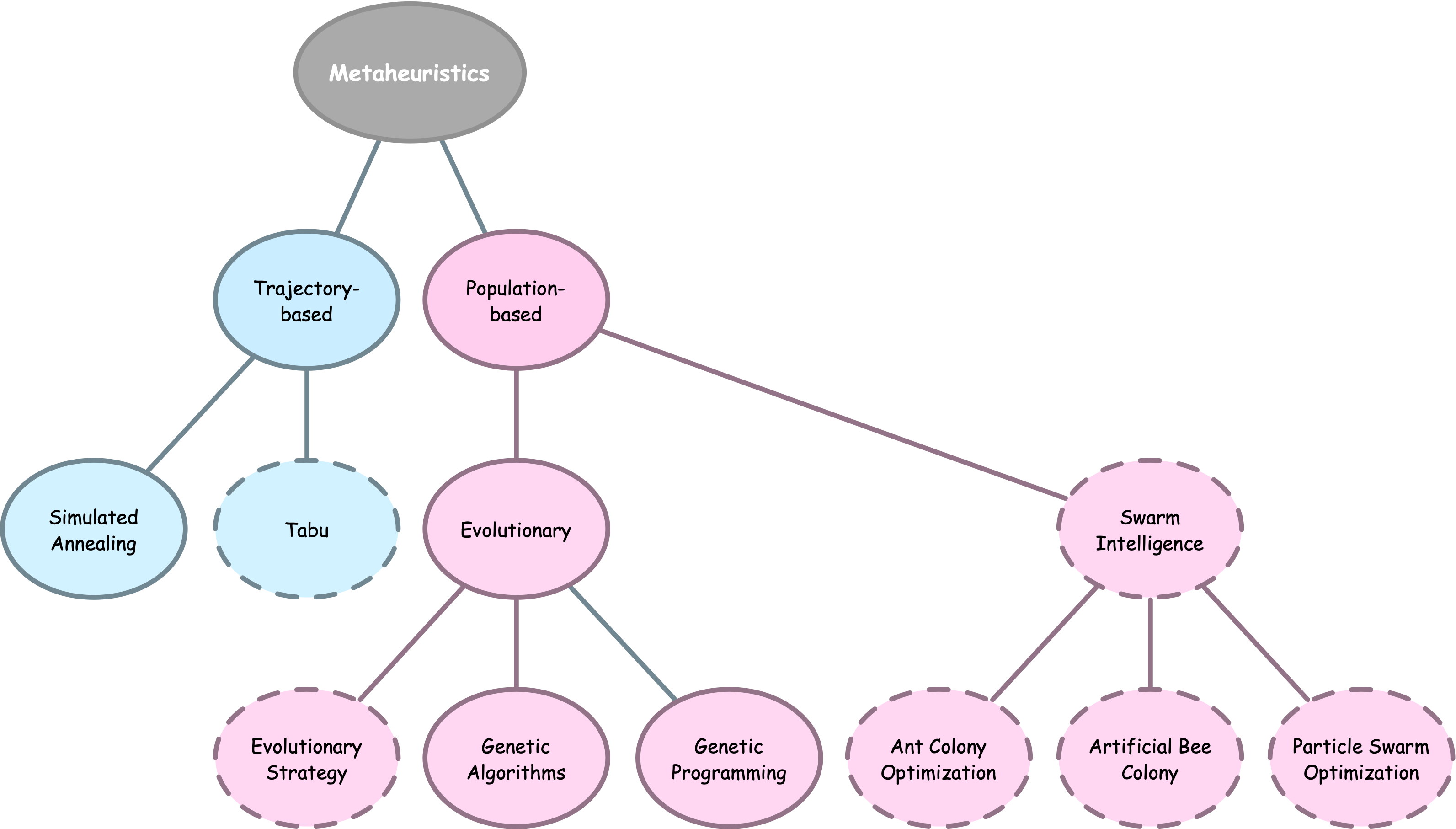
Metaheuristics
Definition
Metaheuristics are higher-level procedures or heuristics designed to guide the search for solutions in optimization problems with large solution spaces, aiming to find good solutions more efficiently than traditional methods.
Meta heuristics balance exploitation and exploration to avoid local optima, often incorporating randomness, memory, or adaptive mechanisms.
Definition
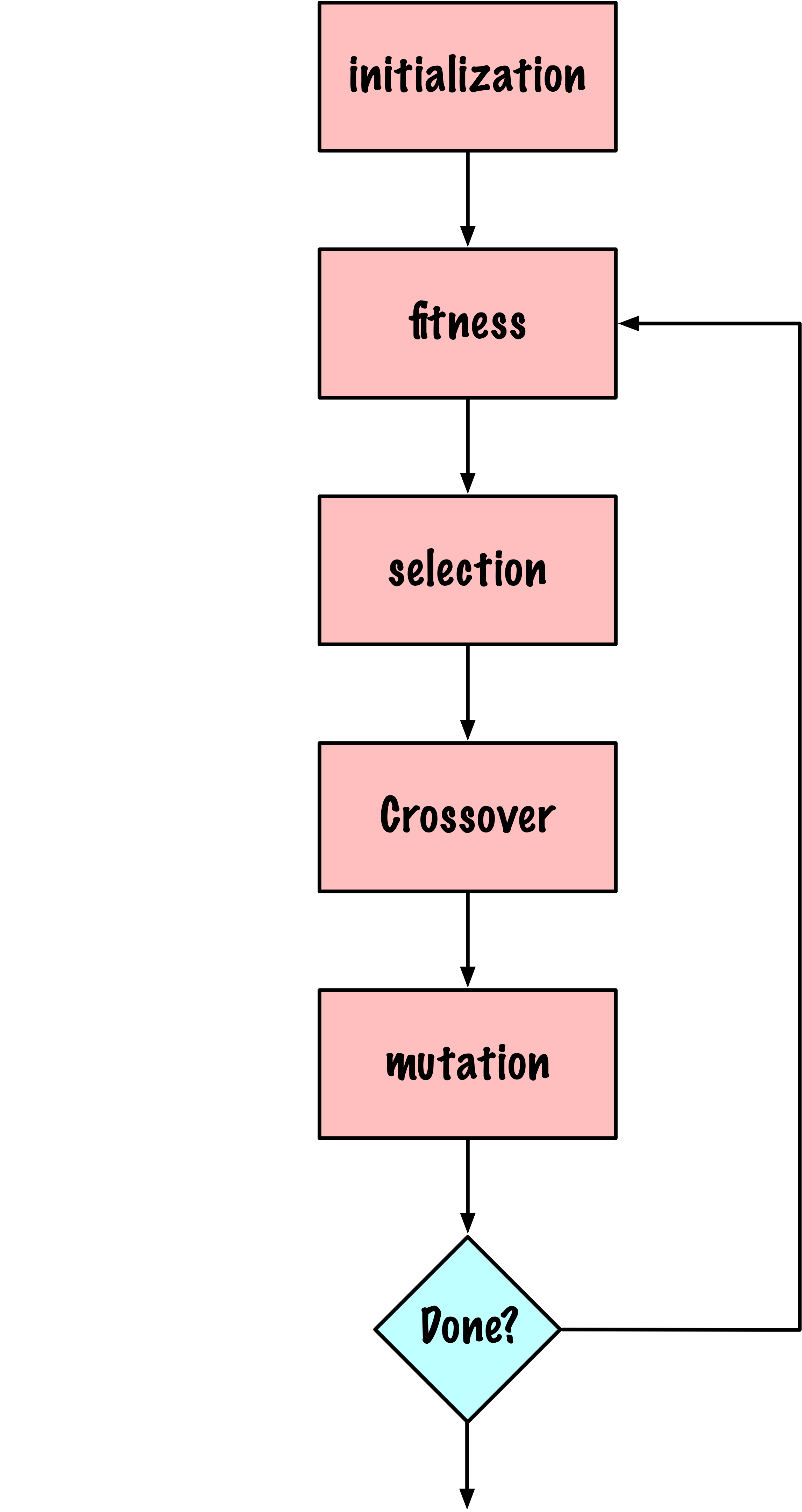
A genetic algorithm is an evolutionary optimization technique that uses a population of candidate solutions, evolving them through selection, crossover, and mutation to iteratively improve towards an “optimal” solution.
Trends in AI
Applications
- Optimization: Solving complex engineering, logistics, and scheduling problems.
- Machine Learning: Feature selection, hyperparameter tuning, and evolving neural network architectures.
- Robotics: Path planning, sensor optimization, control strategy development, and robot designs1.
Applications (continued)
From Biology to Genetic Algorithms
There is probably no more original, more complex, and bolder concept in the history of ideas than Darwin’s mechanistic explanation of adaptation.
If I were to give an award for the single best idea anyone has ever had, I’d give it to Darwin, ahead of Newton & Einstein and everyone else.
Definition
Natural selection is a non-random difference in reproductive output among replicating entities, often due indirectly to differences in survival in a particular environment, leading to an increase in the proportion of beneficial, heritable characteristics within a population from one generation to the next.
Components
Basic GA
Choices
- How to encode a candidate solution or state?
- How to select candidate solutions?
- How to define the crossover operator?
- How to define the mutation operator?
- How to calculate the fitness?
Problem
Problem (continued)
\[ \begin{aligned} & \text { maximize } \sum_{i=1}^n x_i \cdot v_i \\ & \text { subject to } \sum_{i=1}^n x_i \cdot w_i \leq W \text { and } x_i \in\{0,1\} . \end{aligned} \]
where \(W\) represents the fixed maximum weight, and \(x_i\) is a binary variable indicating whether item \(i\) is included (1) or excluded (0).
Applications
Finance and Investment: In portfolio optimization, where each asset has a risk (analogous to weight) and expected return (value), the knapsack framework helps select a set of assets that maximizes return without exceeding a risk threshold.
Resource Allocation: Common in project management, where resources (budget, personnel, time) need to be allocated across projects or tasks to maximize overall value, taking into account limited availability.
Supply Chain and Logistics: Used to maximize the value of goods transported within vehicle weight or volume constraints. It can also be applied in warehouse storage, where space is limited, and high-value items are prioritized.
Ad Placement and Marketing: Used in digital advertising to select the most profitable combination of ads to display within limited space (e.g., website or app banner space), maximizing revenue under size or display constraints.
Greedy Algorithms
Greedy algorithms make the decision of what to do next by selecting the best local option from all available choices without regard to the global structure.
Data
Ascending order of weight
def greedy_knapsack_weight(weights, values, capacity):

    num_items = len(weights)

    # Create a list of items with their values and original indices
    items = list(zip(weights, values, range(num_items)))

    # Sort items by weight in increasing order
    items.sort()

    total_weight, total_value = 0,0
    solution = np.zeros(num_items, dtype=int)

    # Select items based on the sorted order
    for w, v, idx in items:
        if total_weight + w <= capacity:
            solution[idx] = 1
            total_weight += w
            total_value += v
        else:
            break  # Skip items that would exceed the capacity

return solution, total_value, total_weightgreedy_knapsack_weight
solution, total_value, total_weight = greedy_knapsack_weight(weights, values, capacity)

print(f"Solution: {solution}")
print(f"Value: {total_value}")
print(f"Weight: {total_weight}")
Solution: [1 1 1 1 0 0 1 0 0 0 0 1 1 1 1 1 1 1 1 1 1 1 1 1 1 1 1 1 1 0 1 1 1 1 1 1 0
1 0 1 0 0 1 0 1 0 1 0 1 1]
Value: 5891
Weight: 817Descending value order
def greedy_knapsack_value(weights, values, capacity):

    num_items = len(weights)

    # Create a list of items with their values and original indices
    items = list(zip(values, weights, range(num_items)))

    # Sort items by value in decreasing order
    items.sort(reverse=True)

    total_weight = 0
    total_value = 0
    solution = np.zeros(num_items, dtype=int)

    # Select items based on the sorted order
    for v, w, idx in items:
        if total_weight + w <= capacity:
            solution[idx] = 1
            total_weight += w
            total_value += v

return solution, total_value, total_weightgreedy_knapsack_value
solution, total_value, total_weight = greedy_knapsack_value(weights, values, capacity)

print(f"Solution: {solution}")
print(f"Value: {total_value}")
print(f"Weight: {total_weight}")
Solution: [1 1 0 1 1 0 1 0 0 1 1 1 1 0 1 1 0 1 0 1 1 1 1 0 0 0 0 0 0 1 1 0 0 0 1 0 0
0 1 1 0 1 1 0 1 0 0 1 1 1]
Value: 7339
Weight: 849GA Implementation
Encoding
Population
def initialize_population(pop_size, num_items):

    """
    Initialize the population with random binary strings.

    Args:
        pop_size (int): Number of individuals in the population.
        num_items (int): Number of items in the knapsack problem.

    Returns:
        np.ndarray: Initialized population.
    """

return np.random.randint(2, size=(pop_size, num_items))Population
The proposed method for initializing the population presents a problem.
Fitness
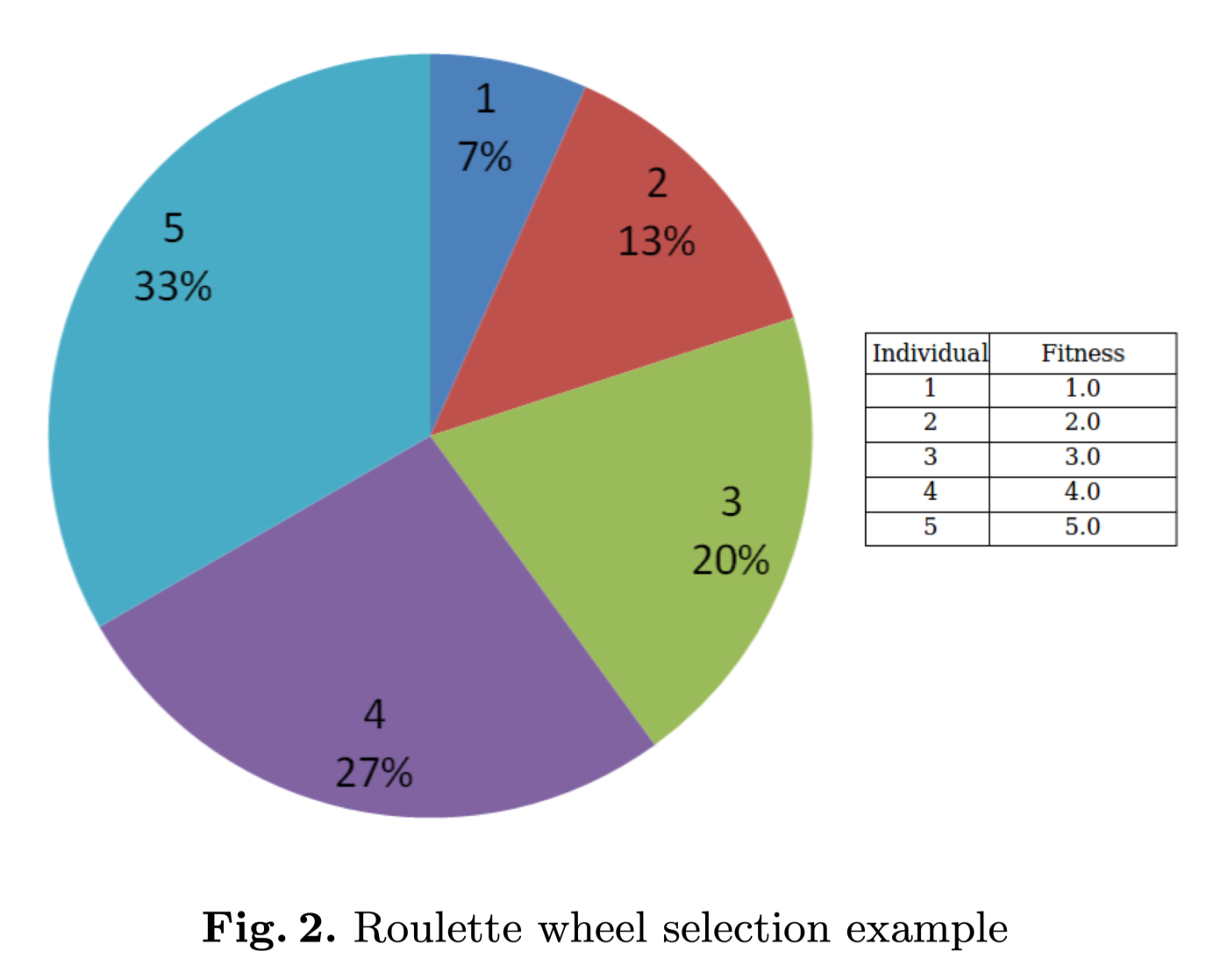
Roulette Wheel Selection
roulette_selection
def roulette_selection(population, fitness):

    # Adjust fitness to be non-negative
    min_fitness = np.min(fitness)
    adjusted_fitness = fitness - min_fitness + 1e-6  # small epsilon to avoid zero division

    total_fitness = np.sum(adjusted_fitness)
    probabilities = adjusted_fitness / total_fitness

    pop_size = population.shape[0]
    selected_indices = np.random.choice(pop_size, size=pop_size, p=probabilities)

return population[selected_indices]Crossover
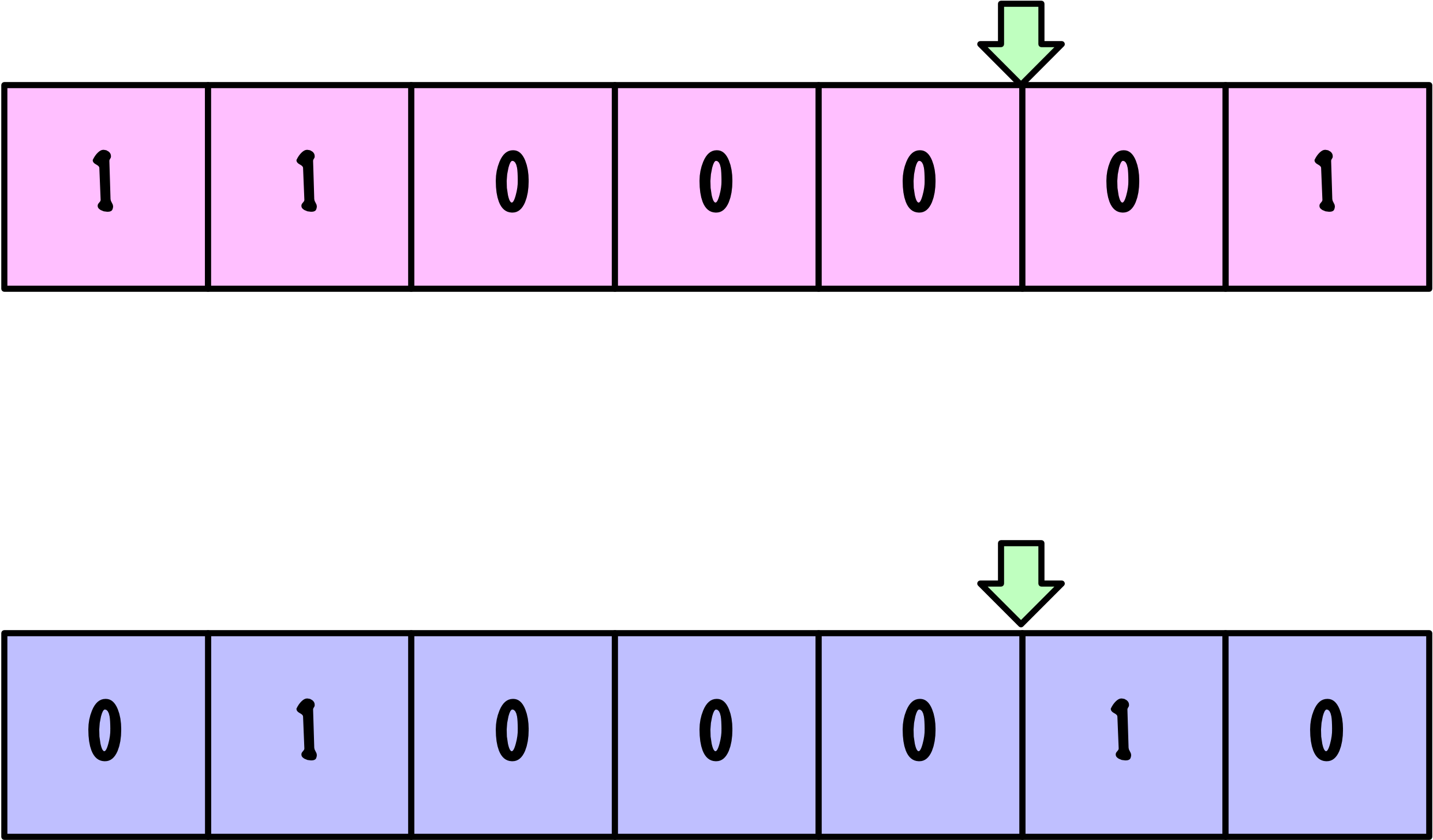
Crossover
Crossover
def single_point_crossover(parents, crossover_rate):

    num_parents, num_genes = parents.shape
    np.random.shuffle(parents)
    offspring = []

    for i in range(0, num_parents, 2):

        parent1 = parents[i]
        parent2 = parents[i+1 if i+1 < num_parents else 0]

        child1 = parent1.copy()
        child2 = parent2.copy()

        if np.random.rand() < crossover_rate:
            point = np.random.randint(1, num_genes)  # Crossover point
            child1[:point], child2[:point] = parent2[:point], parent1[:point]

        offspring.append(child1)
        offspring.append(child2)

return np.array(offspring)Mutation
Mutate
Clarification
np.random.seed(42)

offspring = initialize_population(4, 10)

num_offspring, num_genes = offspring.shape

print("Offspring:")
print(offspring)
Offspring:
[[0 1 0 0 0 1 0 0 0 1]
[0 0 0 0 1 0 1 1 1 0]
[1 0 1 1 1 1 1 1 1 1]
[0 0 1 1 1 0 1 0 0 0]]mutation_rate = 0.05
mutation_matrix = np.random.rand(num_offspring, num_genes) < mutation_rate
print("Mutation matrix:")
print(mutation_matrix)Mutation matrix:
[[False False False False False False False False False True]
[False False False False False False False False False False]
[False False True False False False False False False False]
[False False False False False False False False True False]]offspring[mutation_matrix]:
[1 1 0]1 - offspring[mutation_matrix]:
[0 0 1]Elitism
Elitism in genetic algorithms is a strategy where a subset of the fittest individuals from the current generation is directly carried over to the next generation.
This approach ensures that the best solutions are preserved throughout the evolutionary process, enhancing convergence speed and maintaining high-quality solutions within the population.
Elitism
Genetic Algorithm (Version 1)
def genetic_algorithm(weights, values, capacity, pop_size=100,
                      num_generations=100, crossover_rate=0.8,
                      mutation_rate=0.05, elite_percent=0.02):

    num_items = len(weights)
    elite_size = max(1, int(pop_size * elite_percent))
    population = initialize_population(pop_size, num_items)

    for generation in range(num_generations):

        fitness = evaluate_fitness(population, weights, values, capacity)

        # Elitism
        elites = elitism(population, fitness, elite_size)

        # Selection
        parents = roulette_selection(population, fitness)

        # Crossover
        offspring = single_point_crossover(parents, crossover_rate)

        # Mutation
        offspring = mutation(offspring, mutation_rate)

        # Create new population
        population = np.vstack((elites, offspring))

        # Ensure population size
        if population.shape[0] > pop_size:
            population = population[:pop_size]
        elif population.shape[0] < pop_size:
            # Add random individuals to fill population
            num_new_individuals = pop_size - population.shape[0]
            new_individuals = initialize_population(num_new_individuals, num_items)
            population = np.vstack((population, new_individuals))

    # After all generations, return the best solution
    fitness = evaluate_fitness(population, weights, values, capacity)
    best_index = np.argmax(fitness)
    best_solution = population[best_index]
    best_value = np.dot(best_solution, values)
    best_weight = np.dot(best_solution, weights)

    return best_solution, best_value, best_weight
Run
np.random.seed(13)

solution, total_value, total_weight = genetic_algorithm(weights, values, capacity)

print(f"Solution: {solution}")
print(f"Value: {total_value}")
print(f"Weight: {total_weight}")
Solution: [1 1 0 1 1 0 1 0 0 0 1 1 1 0 1 1 1 1 1 0 1 1 1 0 0 1 0 1 0 1 1 1 1 1 1 0 0
1 0 1 0 0 1 0 1 0 0 1 1 1]
Value: 7357
Weight: 848Genetic Algorithm (Version 1.1)
def genetic_algorithm(weights, values, capacity, pop_size=100,
                      num_generations=100, crossover_rate=0.8,
                      mutation_rate=0.05, elite_percent=0.02):

    num_items = len(weights)
    elite_size = max(1, int(pop_size * elite_percent))
    population = initialize_population(pop_size, num_items)

    average_fitness_history = []
    best_fitness_history = []

    for generation in range(num_generations):

        fitness = evaluate_fitness(population, weights, values, capacity)

        # Track average and best fitness
        average_fitness = np.mean(fitness)
        best_fitness = np.max(fitness)
        average_fitness_history.append(average_fitness)
        best_fitness_history.append(best_fitness)

        # Elitism
        elites = elitism(population, fitness, elite_size)

        # Selection
        parents = roulette_selection(population, fitness)

        # Crossover
        offspring = single_point_crossover(parents, crossover_rate)

        # Mutation
        offspring = mutation(offspring, mutation_rate)

        # Create new population
        population = np.vstack((elites, offspring))

        # Ensure population size
        if population.shape[0] > pop_size:
            population = population[:pop_size]
        elif population.shape[0] < pop_size:
            # Add random individuals to fill population
            num_new_individuals = pop_size - population.shape[0]
            new_individuals = initialize_population(num_new_individuals, num_items)
            population = np.vstack((population, new_individuals))

    # After all generations, return the best solution
    fitness = evaluate_fitness(population, weights, values, capacity)
    best_index = np.argmax(fitness)
    best_solution = population[best_index]
    best_value = np.dot(best_solution, values)
    best_weight = np.dot(best_solution, weights)

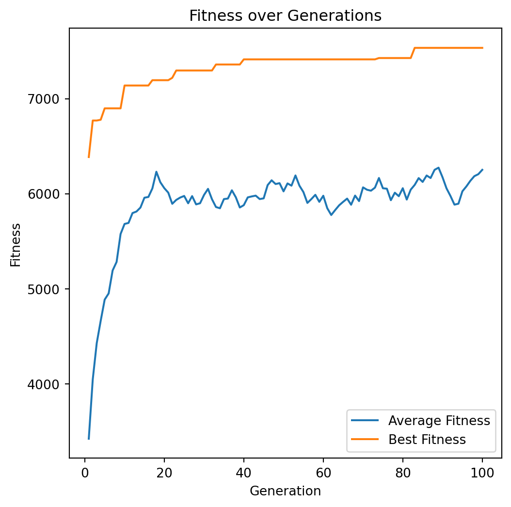
    return best_solution, best_value, best_weight, average_fitness_history, best_fitness_history
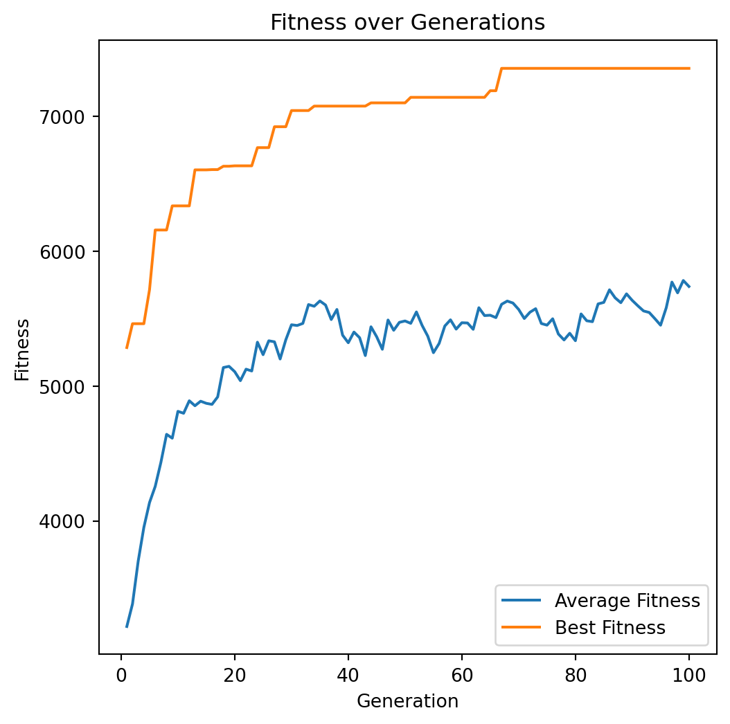
Plot
import matplotlib.pyplot as plt

def plot_fitness_over_generations(avg_fitness_history, best_fitness_history):

  generations = range(1, len(avg_fitness_history) + 1)

  plt.figure(figsize=(6, 6))

  plt.plot(generations, avg_fitness_history, label='Average Fitness')
  plt.plot(generations, best_fitness_history, label='Best Fitness')
  plt.xlabel('Generation')
  plt.ylabel('Fitness')
  plt.title('Fitness over Generations')
  plt.legend()
Run
np.random.seed(13)

solution, total_value, total_weight, avg_fitness_history, best_fitness_history = genetic_algorithm(weights, values, capacity)

print(f"Solution: {solution}")
print(f"Value: {total_value}")
print(f"Weight: {total_weight}")

plot_fitness_over_generations(avg_fitness_history, best_fitness_history)
Run
Run
np.random.seed(42)

best_value = -1
best_weight = -1
best_solution, best_averages, best_bests = None,  None, None

for i in range(100):

  solution, total_value, total_weight, avg_fitness_history, best_fitness_history = genetic_algorithm(weights, values, capacity)

  if total_value > best_value and total_weight <= capacity:
    best_value = total_value
    best_weight = total_weight
    best_solution = solution
    best_averages = avg_fitness_history
    best_bests = best_fitness_history


print(f"Solution: {best_solution}")
print(f"Value: {best_value}")
print(f"Weight: {best_weight}")

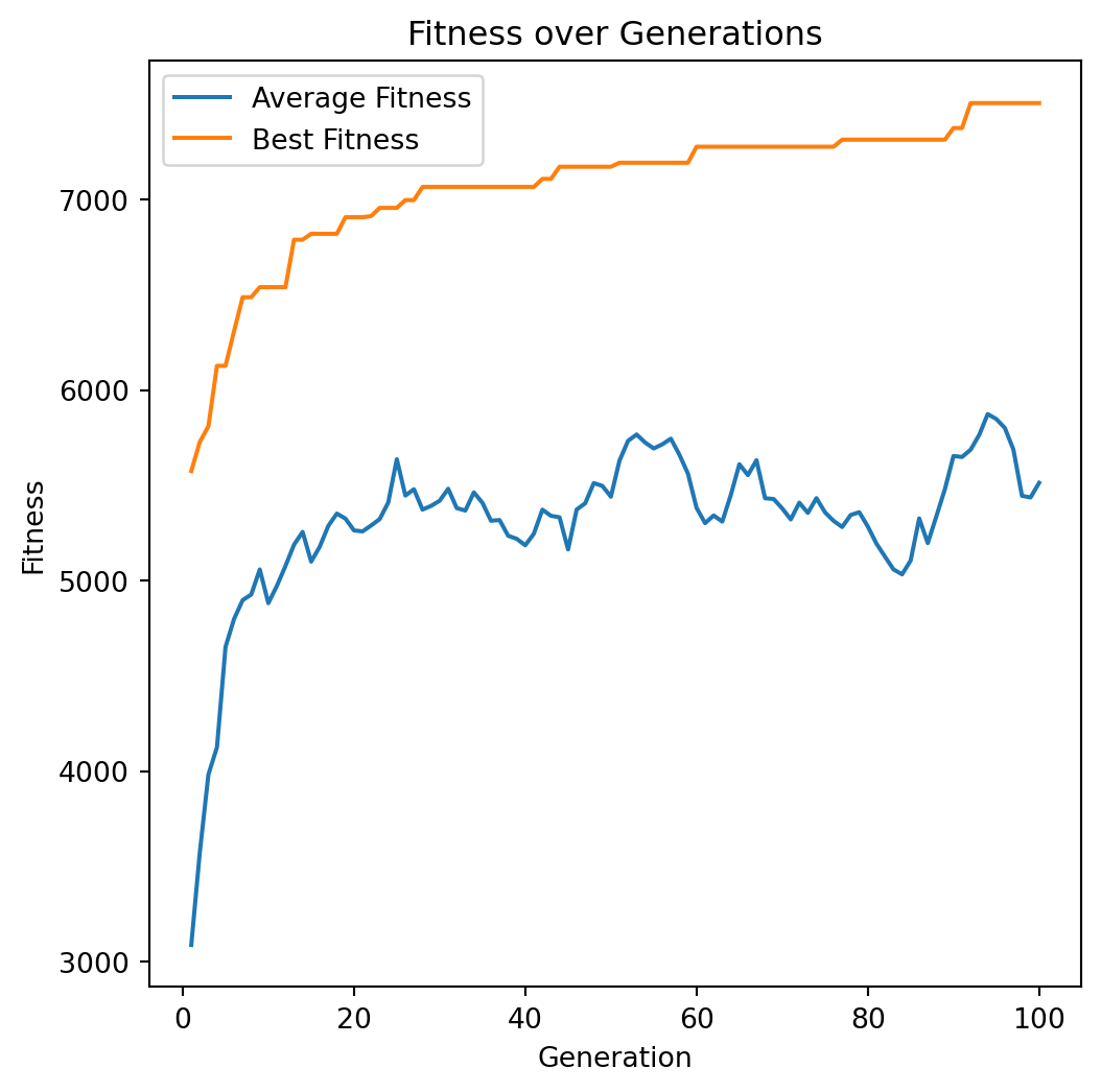
plot_fitness_over_generations(best_averages, best_bests)
Run
Using Google OR Tools
# https://developers.google.com/optimization/pack/knapsack

from ortools.algorithms.python import knapsack_solver

def solve_using_ortools(values, weights, capacity):

  weights = [weights]

  # Create the solver

  solver = knapsack_solver.KnapsackSolver(
      knapsack_solver.SolverType.KNAPSACK_MULTIDIMENSION_BRANCH_AND_BOUND_SOLVER,
      "KnapsackExample",
  )

  solver.init(values, weights, [capacity])

  computed_value = solver.solve()

  packed_items = []
  packed_weights = []
  total_weight = 0
  print("Total value =", computed_value)
  for i in range(len(values)):
      if solver.best_solution_contains(i):
          packed_items.append(i)
          packed_weights.append(weights[0][i])
          total_weight += weights[0][i]
  print("Total weight:", total_weight)
  print("Packed items:", packed_items)
  print("Packed_weights:", packed_weights)
solve_using_ortools
Total value = 7534
Total weight: 850
Packed items: [0, 1, 3, 4, 6, 10, 11, 12, 14, 15, 16, 17, 18, 19, 21, 22, 24, 27, 28, 29, 30, 31, 32, 34, 38, 39, 41, 42, 44, 47, 48, 49]
Packed_weights: [7, 0, 22, 80, 11, 59, 18, 0, 3, 8, 15, 42, 9, 0, 47, 52, 26, 6, 29, 84, 2, 4, 18, 7, 71, 3, 66, 31, 0, 65, 52, 13]
Discussion
Encoding Schemes
Binary encoding is commonly used.
Permutation encoding. Typically used with problems such as “Travelling Salesman Problem (TSP)” and N-Queens.
Values encoding. In this encoding, integer, real, or character values are used. Example: learning the parameters of a polynomical in a regression problem.
Selection
Tournament selection involves randomly selecting a subset of individuals (a tournament) from the population and then selecting the best individual from this subset to be a parent. The process is repeated until the required number of parents is selected.
This method balances between exploration and exploitation. It allows for controlling selection pressure by varying the tournament size. Larger tournaments increase selection pressure, favoring the fittest individuals more strongly.
tournament_selection
def tournament_selection(population, fitness, tournament_size):

    pop_size = population.shape[0]

    selected_indices = []

    for _ in range(pop_size):

        participants = np.random.choice(pop_size, tournament_size, replace=False)

        best = participants[np.argmax(fitness[participants])]

        selected_indices.append(best)

return population[selected_indices]Discussion
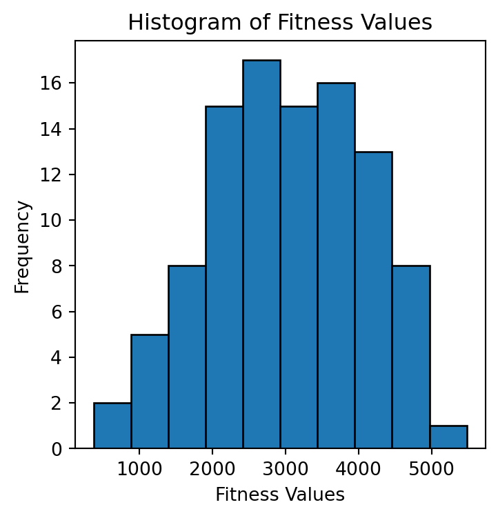
np.random.seed(27)

pop_size, num_items = 100, 50

population = initialize_population(pop_size, num_items)

fitness = evaluate_fitness(population, weights, values, capacity)

plt.figure(figsize=(4, 4))
plt.hist(fitness, bins=10, edgecolor='black')
plt.xlabel('Fitness Values')
plt.ylabel('Frequency')
plt.title('Histogram of Fitness Values')
plt.show()

for tournament_size in [2, 4, 8, pop_size]:
  participants = np.random.choice(pop_size, tournament_size, replace=False)
print(f"tournament_size: {tournament_size}, fitness: {max(fitness[participants])}")Discussion
Genetic Algorithm (Version 2)
def genetic_algorithm(weights, values, capacity, pop_size=100,
                      num_generations=100, crossover_rate=0.8,
                      mutation_rate=0.05, elite_percent=0.02,
                      selection_type='tournament', tournament_size=3):

    num_items = len(weights)
    elite_size = max(1, int(pop_size * elite_percent))
    population = initialize_population(pop_size, num_items)

    average_fitness_history = []
    best_fitness_history = []

    for generation in range(num_generations):

        fitness = evaluate_fitness(population, weights, values, capacity)

        # Track average and best fitness
        average_fitness = np.mean(fitness)
        best_fitness = np.max(fitness)
        average_fitness_history.append(average_fitness)
        best_fitness_history.append(best_fitness)

        # Elitism
        elites = elitism(population, fitness, elite_size)

        # Selection
        if selection_type == 'tournament':
            parents = tournament_selection(population, fitness, tournament_size)
        elif selection_type == 'roulette':
            parents = roulette_selection(population, fitness)
        else:
            raise ValueError("Invalid selection type")

        # Crossover
        offspring = single_point_crossover(parents, crossover_rate)

        # Mutation
        offspring = mutation(offspring, mutation_rate)

        # Create new population
        population = np.vstack((elites, offspring))

        # Ensure population size
        if population.shape[0] > pop_size:
            population = population[:pop_size]
        elif population.shape[0] < pop_size:
            # Add random individuals to fill population
            num_new_individuals = pop_size - population.shape[0]
            new_individuals = initialize_population(num_new_individuals, num_items)
            population = np.vstack((population, new_individuals))

    # After all generations, return the best solution
    fitness = evaluate_fitness(population, weights, values, capacity)
    best_index = np.argmax(fitness)
    best_solution = population[best_index]
    best_value = np.dot(best_solution, values)
    best_weight = np.dot(best_solution, weights)

    return best_solution, best_value, best_weight, average_fitness_history, best_fitness_history
Run
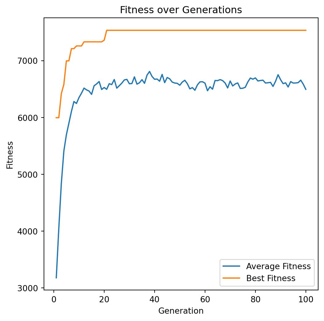
np.random.seed(42)

best_value, best_weight = -1, -1
best_solution, best_averages, best_bests = None,  None, None

for i in range(100):

  solution, total_value, total_weight, avg_fitness_history, best_fitness_history = genetic_algorithm(weights, values, capacity)

  if total_value > best_value and total_weight <= capacity:
    best_value = total_value
    best_weight = total_weight
    best_solution = solution
    best_averages = avg_fitness_history
    best_bests = best_fitness_history


print(f"Solution: {best_solution}")
print(f"Value: {best_value}")
print(f"Weight: {best_weight}")

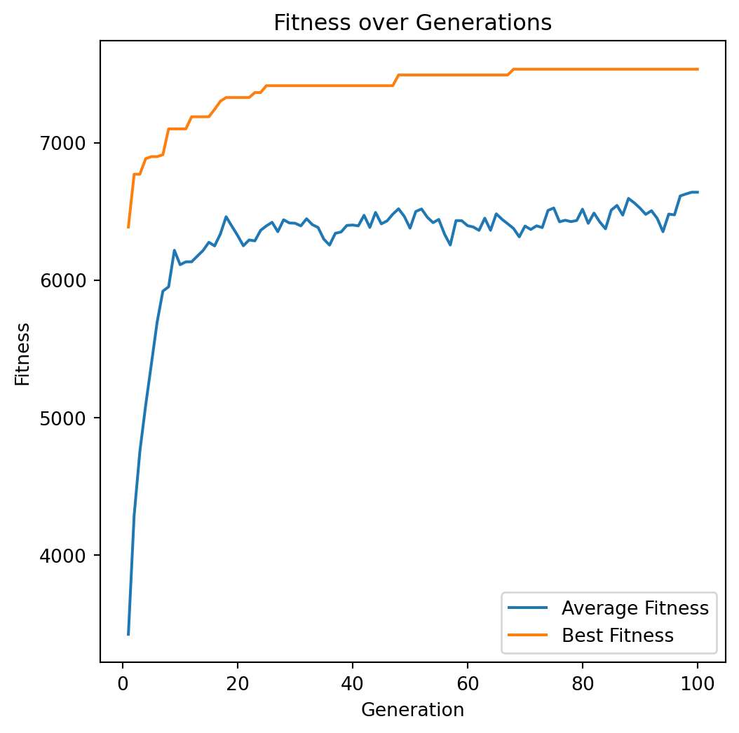
plot_fitness_over_generations(best_averages, best_bests)
Run
tournament_size=2, 4, 8
np.random.seed(42)
for tournament_size in (2, 4, 8):
best_value, best_weight = -1, -1
best_solution, best_averages, best_bests = None, None, None
for i in range(100):
solution, total_value, total_weight, avg_fitness_history, best_fitness_history = genetic_algorithm(
weights, values, capacity, tournament_size=tournament_size
)
if total_value > best_value and total_weight <= capacity:
best_value = total_value
best_weight = total_weight
best_solution = solution
best_averages = avg_fitness_history
best_bests = best_fitness_history
print(f"Solution: {best_solution}")
print(f"Value: {best_value}")
print(f"Weight: {best_weight}")
plot_fitness_over_generations(best_averages, best_bests)tournament_size=2, 4, 8
Solution: [1 1 0 1 1 0 1 0 0 0 1 1 1 0 1 1 1 1 1 1 0 1 1 0 1 0 0 1 1 1 1 1 1 0 1 0 0
 0 1 1 0 1 1 0 1 0 0 1 1 1]
Value: 7534
Weight: 850
Solution: [1 1 0 1 1 0 1 0 0 0 1 1 1 0 1 1 1 1 1 1 0 1 1 0 1 0 0 1 1 1 1 1 1 0 1 0 0
0 1 1 0 1 1 0 1 0 0 1 1 1]
Value: 7534
Weight: 850
Solution: [1 1 0 1 1 0 1 0 0 0 1 1 1 0 1 1 1 1 1 1 0 1 1 0 1 0 0 1 1 1 1 1 1 0 1 0 0
0 1 1 0 1 1 0 1 0 0 1 1 1]
Value: 7534
Weight: 850Crossover
- Single or k-point cross-over.
Uniform crossover
Uniform crossover in genetic algorithms is a recombination technique where each gene in the offspring is independently chosen from one of the two parent genomes with equal probability. This approach allows for a more varied combination of parental traits compared to traditional crossover methods, promoting greater genetic diversity in the resulting population.
uniform_crossover
def uniform_crossover(parents, crossover_rate):

    num_parents, num_genes = parents.shape
    np.random.shuffle(parents)

    offspring = []

    for i in range(0, num_parents, 2):

        parent1 = parents[i]
        parent2 = parents[i+1 if i+1 < num_parents else 0]

        child1 = parent1.copy()
        child2 = parent2.copy()

        if np.random.rand() < crossover_rate:

            mask = np.random.randint(0, 2, size=num_genes).astype(bool)

            child1[mask], child2[mask] = parent2[mask], parent1[mask]

        offspring.append(child1)
        offspring.append(child2)

    return np.array(offspring)
Genetic Algorithm (Version 3)
def genetic_algorithm(weights, values, capacity, pop_size=100,
                      num_generations=200, crossover_rate=0.8,
                      mutation_rate=0.05, elite_percent=0.02,
                      selection_type='tournament', tournament_size=3,
                      crossover_type='single_point'):

    num_items = len(weights)
    elite_size = max(1, int(pop_size * elite_percent))
    population = initialize_population(pop_size, num_items)

    average_fitness_history = []
    best_fitness_history = []

    for generation in range(num_generations):

        fitness = evaluate_fitness(population, weights, values, capacity)

        # Track average and best fitness
        average_fitness = np.mean(fitness)
        best_fitness = np.max(fitness)
        average_fitness_history.append(average_fitness)
        best_fitness_history.append(best_fitness)

        # Elitism
        elites = elitism(population, fitness, elite_size)

        # Selection
        if selection_type == 'tournament':
            parents = tournament_selection(population, fitness, tournament_size)
        elif selection_type == 'roulette':
            parents = roulette_selection(population, fitness)
        else:
            raise ValueError("Invalid selection type")

        # Crossover
        if crossover_type == 'single_point':
            offspring = single_point_crossover(parents, crossover_rate)
        elif crossover_type == 'uniform':
            offspring = uniform_crossover(parents, crossover_rate)
        else:
            raise ValueError("Invalid crossover type")

        # Mutation
        offspring = mutation(offspring, mutation_rate)

        # Create new population
        population = np.vstack((elites, offspring))

        # Ensure population size
        if population.shape[0] > pop_size:
            population = population[:pop_size]
        elif population.shape[0] < pop_size:
            # Add random individuals to fill population
            num_new_individuals = pop_size - population.shape[0]
            new_individuals = initialize_population(num_new_individuals, num_items)
            population = np.vstack((population, new_individuals))

    # After all generations, return the best solution
    fitness = evaluate_fitness(population, weights, values, capacity)
    best_index = np.argmax(fitness)
    best_solution = population[best_index]
    best_value = np.dot(best_solution, values)
    best_weight = np.dot(best_solution, weights)

    return best_solution, best_value, best_weight, average_fitness_history, best_fitness_history
Run
np.random.seed(42)

best_value, best_weight = -1, -1
best_solution, best_averages, best_bests = None,  None, None

for i in range(100):

  solution, total_value, total_weight, avg_fitness_history, best_fitness_history = genetic_algorithm(
    weights, values, capacity, crossover_type='uniform'
  )

  if total_value > best_value and total_weight <= capacity:
    best_value = total_value
    best_weight = total_weight
    best_solution = solution
    best_averages = avg_fitness_history
    best_bests = best_fitness_history


print(f"Solution: {best_solution}")
print(f"Value: {best_value}")
print(f"Weight: {best_weight}")

plot_fitness_over_generations(best_averages, best_bests)
Run
Crossover
Single-Point Crossover is advantageous when building blocks (contiguous gene sequences) are meaningful and beneficial to preserve. However, in the 0/1 Knapsack Problem, the position of items in the chromosome is typically arbitrary, and preserving contiguous sections may not correspond to better solutions.
Uniform Crossover offers better exploration by independently mixing genes, which aligns well with the nature of the knapsack problem where each item’s inclusion is an independent decision. It reduces positional bias and increases the likelihood of discovering optimal combinations of items.
Crossover
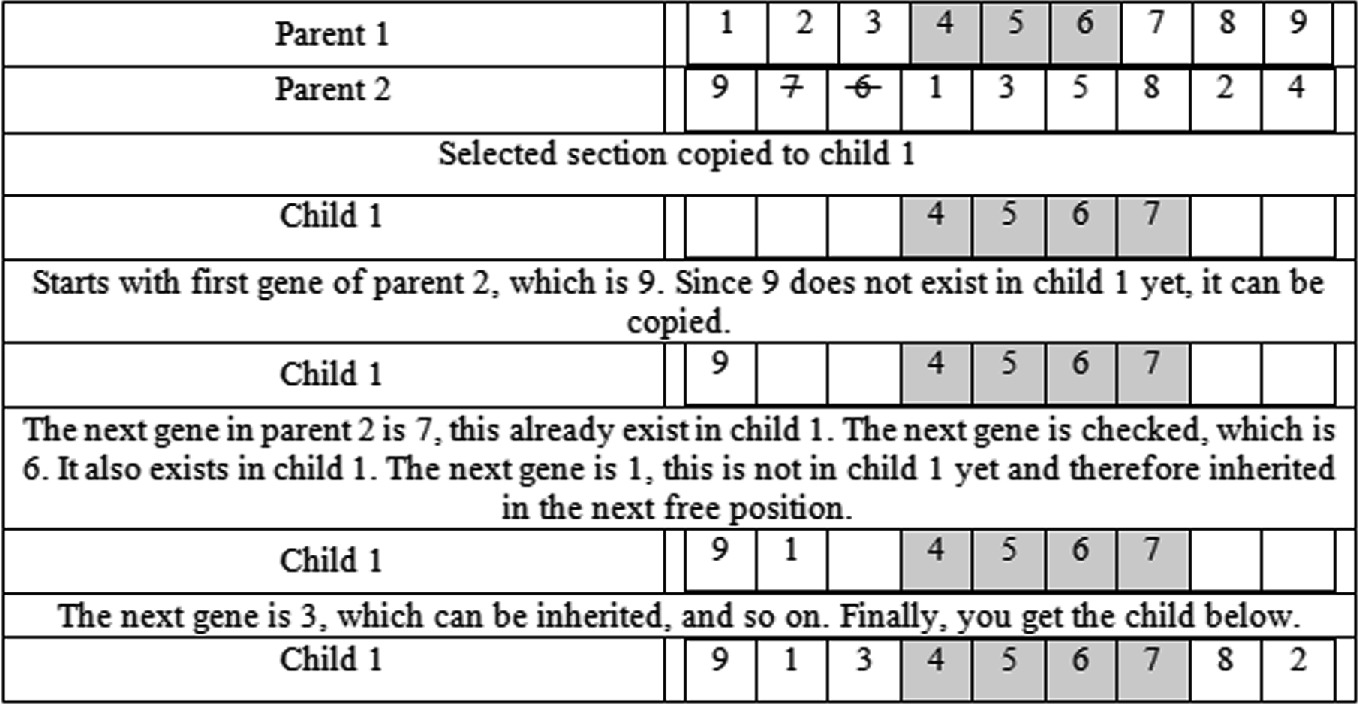
Order preserving. For each offspring, retain the sequence of elements from one parent while filling in the remaining positions with elements from the other parent, preserving their order as they appear in the second parent.
Order 1 crossover (OX)
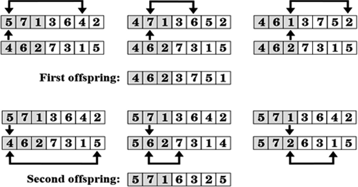
Partially Mapped Crossover (PMX)
Comparison
| Feature | PMX | OX |
|---|---|---|
| Preservation of Position | High | Low |
| Preservation of Order | Partial | High |
| Exploration vs. Exploitation | Exploitation-focused | Exploration-focused |
| Implementation Complexity | Higher | Lower |
| Application Suitability | Problems with positional dependencies | Problems with order dependencies |
Mutation
Bit Flip Mutation: This involves flipping the value of a bit at a selected position within the chromosome.
- Mutation Rate: A typical mutation rate is \(1/n\), where \(n\) represents the length of the chromosome.
Mutation
- Replacement or Random Resetting: For integer and real-valued chromosomes, employ a random selection from the uniform distribution \(U(a, b)\) to choose a new value within the interval \([a, b]\). Similar to the bit flip operator, determine for each position whether a mutation should occur, then apply the replacement if necessary.
Mutation
- Swap Mutation: This operator randomly selects two genes within a permutation and exchanges their positions. Such mutations facilitate the exploration of various permutations, potentially yielding improved solutions.
Remarks
When designing operators, it is critical to ensure they can explore the entire state space exhaustively.
Mutation operators should remain unbiased to maintain the integrity of the exploration process.
Comprehensive Example (1)
A Jupyter Notebook containing all lecture code has been created.
It includes tests on 25 problem instances.
In this context, the genetic algorithm consistently outperformed the greedy algorithms, matching the best greedy results in 8 cases and surpassing them in 17 cases, with improvements up to 6%.
Comprehensive Example (2)
Fredj Kharroubi conducted an empirical study on the knapsack problem, comparing the performance of several algorithms: generate-and-test, greedy search, simulated annealing, and a genetic algorithm.
Discussions on Hyperparameters
Population Size
A larger size improves genetic diversity but increases computational cost.
A smaller size speeds up execution but risks premature convergence.
Discussions on Hyperparameters
Mutation and Crossover Rates
High rates promote exploration but risk disrupting viable solutions.
Low rates favor exploitation but risk getting stuck in local optima.
Discussions on Hyperparameters
Selection and Tournament Size
Tournament selection is robust against uneven fitness distributions.
A medium tournament size (3-5) balances exploration and exploitation well.
Parameters
Genetic algorithms, like many machine learning and search algorithms, require hyperparameter tuning to optimize their performance.
Key hyperparameters in genetic algorithms include population size, mutation rate, crossover rate, selection method, and the number of generations.
Discussion
Like other metaheuristic approaches, genetic algorithms can become trapped in local optima. A common solution, akin to the random restart technique used in hill climbing, is to periodically reinitialize the algorithm to explore different regions of the solution space.
Doubling the population size with each restart enhances the likelihood of exploring diverse regions of the state space.
Skepticism toward GA
[I]t is quite unnatural to model applications in terms of genetic operators like mutation and crossover on bit strings. The pseudobiology adds another level of complexity between you and your problem. Second, genetic algorithms take a very long time on nontrivial problems. [\(\ldots\)] [T]he analogy with evolution – where significant progress require [sic] millions of years – can be quite appropriate. […]
I have never encountered any problem where genetic algorithms seemed to me the right way to attack it. Further, I have never seen any computational results reported using genetic algorithms that have favorably impressed me. Stick to simulated annealing for your heuristic search voodoo needs.
Greedy: value-to-weight ratio
def greedy_knapsack_ratio(weights, values, capacity):

    num_items = len(weights)

    # Calculate value-to-weight ratio for each item
    ratio = values / (weights + 1e-6)

    # Create a list of items with their ratios and original indices
    items = list(zip(ratio, values, weights, range(num_items)))

    # Sort items by ratio in decreasing order
    items.sort(reverse=True)

    total_weight = 0
    total_value = 0
    solution = np.zeros(num_items, dtype=int)

    # Select items based on the sorted order
    for r, v, w, idx in items:
        if total_weight + w <= capacity:
            solution[idx] = 1
            total_weight += w
            total_value += v

return solution, total_value, total_weightgreedy_knapsack_ratio
solution, total_value, total_weight = greedy_knapsack_ratio(weights, values, capacity)

print(f"Solution: {solution}")
print(f"Value: {total_value}")
print(f"Weight: {total_weight}")
Solution: [1 1 0 1 1 0 1 0 0 0 1 1 1 0 1 1 1 1 1 1 0 1 1 0 1 0 0 1 1 1 1 1 1 0 1 0 0
0 1 1 0 1 1 0 1 0 0 1 1 1]
Value: 7534
Weight: 850Frameworks
- DEAP,
- DEAP is an evolutionary computation framework designed for rapid prototyping and testing of ideas. It aims to make algorithms explicit and data structures transparent. The framework seamlessly integrates with parallelization mechanisms, including multiprocessing and SCOOP.
- It has been developed at Université Laval since 2012.
- PyGAD, 5 PyGAD applications
Genetic Programming
Definition
Genetic programming is an evolutionary algorithm-based methodology that evolves computer programs to solve problems by mimicking natural selection processes.
It automatically discovers optimal or near-optimal solutions by iteratively modifying a population of candidate programs, guided by a fitness function.
Genetic Programming
Genetic Programming
Prologue
Conclusion
- Rather than exploring a single solution at a time, GA explore several solutions in parallel.
Comparison of SA and GA
| Aspect | Simulated Annealing (SA) | Genetic Algorithms (GA) |
|---|---|---|
| Solution Representation | Single solution iteratively improved | Population of solutions evolved over generations |
| Exploration Mechanism | Random moves to neighboring solutions; acceptance based on temperature | Crossover and mutation generate new solutions from existing ones |
| Exploitation Mechanism | Gradual reduction in temperature focuses search around current best solution | Selection and elitism favor fitter individuals in the population |
| Control Parameters | Temperature, cooling schedule | Population size, crossover rate, mutation rate, selection method |
| Search Strategy | Explores by accepting worse solutions at higher temperatures | Explores by combining and mutating existing solutions |
| Balance of Exploration and Exploitation | Controlled by temperature schedule | Controlled by genetic operator rates and selection pressure |
| Escape from Local Optima | Possible due to probabilistic acceptance of worse solutions | Possible due to diversity in population and genetic variations |
| Convergence | Depends on cooling schedule; may be slow for large problems | Can converge prematurely without sufficient diversity |
Summary
Metaheuristics Overview
Genetic Algorithms (GAs)
Applications of GAs
Components of GAs:
- Encoding: Representation of candidate solutions (e.g., binary strings for the knapsack problem).
- Population: A set of candidate solutions initialized randomly or by some heuristic.
- Selection: Methods like roulette wheel and tournament selection choose fitter individuals for reproduction.
- Crossover: Combines parts of two parents to create offspring (e.g., single-point crossover).
- Mutation: Randomly alters genes in a chromosome to maintain genetic diversity.
- Fitness Function: Evaluates how close a candidate solution is to the optimum.
Knapsack Problem Example:
- Demonstrated how to apply GAs to the 0/1 knapsack problem.
- Provided Python code snippets implementing GA components for the problem.
- Showed how to generate an initial population, perform crossover and mutation, and select the next generation.
- Compared GA solutions with optimal solutions obtained using Google’s OR-Tools.
Further Readings
Resources
See Direct Evolutionary Optimization of Variational Autoencoders With Binary Latents for a recent application in machine learning.
Next lecture
- We will look at the Monte Carlo Tree Search (MCTS) algorithm
References
Marcel Turcotte
School of Electrical Engineering and Computer Science (EECS)
University of Ottawa
