Model Evaluation and Hyperparameter Tuning

CSI 4106 - Fall 2024

Author

Marcel Turcotte

Published

Version: Nov 14, 2024 09:02

Preamble

Quote of the Day

Super Intelligence from The Future with Hannah Fry aired September 12th, 2024.

Learning Objectives

Understand the Purpose of Data Splitting:
- Describe the roles of the training, validation, and test sets in model evaluation.
- Explain why and how datasets are divided for effective model training and evaluation.
Explain Cross-Validation Techniques:
- Define cross-validation and its importance in model evaluation.
- Illustrate the process of \(k\)-fold cross-validation and its advantages over a single train-test split.
- Discuss the concepts of underfitting and overfitting in the context of cross-validation.
Hyperparameter Tuning:
- Explain the difference between model parameters and hyperparameters.
- Describe methods for tuning hyperparameters, including grid search and randomized search.
- Implement hyperparameter tuning using GridSearchCV in scikit-learn.
Evaluate Model Performance:
- Interpret cross-validation results and understand metrics like mean and standard deviation of scores.
- Discuss how cross-validation helps in assessing model generalization and reducing variability.
Machine Learning Engineering Workflow:
- Outline the steps involved in preparing data for machine learning models.
- Utilize scikit-learn pipelines for efficient data preprocessing and model training.
- Emphasize the significance of consistent data transformations across training and production environments.
Critical Evaluation of Machine Learning Models:
- Assess the limitations and challenges associated with hyperparameter tuning and model selection.
- Recognize potential pitfalls in data preprocessing, such as incorrect handling of missing values or inconsistent encoding.
- Advocate for thorough testing and validation to ensure model reliability and generalizability.
Integrate Knowledge in Practical Applications:
- Apply the learned concepts to real-world datasets (e.g., OpenML datasets like ‘diabetes’ and ‘adult’).
- Interpret and analyze the results of model evaluations and experiments.
- Develop a comprehensive understanding of the end-to-end machine learning pipeline.

The above learning objectives have been generated by OpenAI’s model, o1, based on the lecture content.

Introduction

Dataset - openml

www.openml.org

OpenML is an open platform for sharing datasets, algorithms, and experiments - to learn how to learn better, together.

. . .

import numpy as np
np.random.seed(42)

from sklearn.datasets import fetch_openml

diabetes = fetch_openml(name='diabetes', version=1)
print(diabetes.DESCR)

Author: Vincent Sigillito

Source: Obtained from UCI

Please cite: UCI citation policy

Title: Pima Indians Diabetes Database
Sources:
1. Original owners: National Institute of Diabetes and Digestive and Kidney Diseases
2. Donor of database: Vincent Sigillito ([email protected]) Research Center, RMI Group Leader Applied Physics Laboratory The Johns Hopkins University Johns Hopkins Road Laurel, MD 20707 (301) 953-6231
3. Date received: 9 May 1990
Past Usage:
1. Smith,_J.W., Everhart,_J.E., Dickson,_W.C., Knowler,_W.C., & Johannes,_R.S. (1988). Using the ADAP learning algorithm to forecast the onset of diabetes mellitus. In {it Proceedings of the Symposium on Computer Applications and Medical Care} (pp. 261–265). IEEE Computer Society Press.
  
  The diagnostic, binary-valued variable investigated is whether the patient shows signs of diabetes according to World Health Organization criteria (i.e., if the 2 hour post-load plasma glucose was at least 200 mg/dl at any survey examination or if found during routine medical care). The population lives near Phoenix, Arizona, USA.
  
  Results: Their ADAP algorithm makes a real-valued prediction between 0 and 1. This was transformed into a binary decision using a cutoff of 0.448. Using 576 training instances, the sensitivity and specificity of their algorithm was 76% on the remaining 192 instances.
Relevant Information: Several constraints were placed on the selection of these instances from a larger database. In particular, all patients here are females at least 21 years old of Pima Indian heritage. ADAP is an adaptive learning routine that generates and executes digital analogs of perceptron-like devices. It is a unique algorithm; see the paper for details.
Number of Instances: 768
Number of Attributes: 8 plus class
For Each Attribute: (all numeric-valued)
1. Number of times pregnant
2. Plasma glucose concentration a 2 hours in an oral glucose tolerance test
3. Diastolic blood pressure (mm Hg)
4. Triceps skin fold thickness (mm)
5. 2-Hour serum insulin (mu U/ml)
6. Body mass index (weight in kg/(height in m)^2)
7. Diabetes pedigree function
8. Age (years)
9. Class variable (0 or 1)
Missing Attribute Values: None
Class Distribution: (class value 1 is interpreted as “tested positive for diabetes”)

Class Value Number of instances 0 500 1 268

Brief statistical analysis:

Attribute number: Mean: Standard Deviation:

```
                3.8     3.4
```
```
              120.9    32.0
```
```
               69.1    19.4
```
```
               20.5    16.0
```
```
               79.8   115.2
```
```
               32.0     7.9
```
```
                0.5     0.3
```
```
               33.2    11.8
```

Relabeled values in attribute ‘class’ From: 0 To: tested_negative
From: 1 To: tested_positive

Downloaded from openml.org.

Today’s dataset is the PIMA dataset, which contains 768 instances and 8 numerical attributes. The numerical nature of these attributes facilitates our analysis. Additionally, since the data originates from a published paper, it likely reflects careful data collection, potentially leading to robust results, as the authors would have needed high-quality data to support their publication.

Dataset - `return_X_y`

fetch_openml returns a Bunch, a DataFrame, or X and y

from sklearn.datasets import fetch_openml

X, y = fetch_openml(name='diabetes', version=1, return_X_y=True)

. . .

Mild imbalance (ratio less than 3 or 4)

print(y.value_counts())

class
tested_negative    500
tested_positive    268
Name: count, dtype: int64

. . .

Converting the target labels to 0 and 1

y = y.map({'tested_negative': 0, 'tested_positive': 1})

Cross-evaluation

Training and test set

Sometimes called holdout method.

Guideline: Typically, allocate 80% of your dataset for training and reserve the remaining 20% for testing.
Training Set: This subset of data is utilized to train your model.
Test Set: This is an independent subset used exclusively at the final stage to assess the model’s performance.

Common Training and Testing Ratios

80:20 Split:
- Training Set: 80% of the data
- Testing Set: 20% of the data
- This is a widely used default split that provides a balance between having enough data to train the model and enough data to evaluate its performance.
90:10 Split:
- Training Set: 90% of the data
- Testing Set: 10% of the data
- This split might be used when the dataset is very large, ensuring a substantial amount of data for training while still having a decent-sized test set.

Considerations for Choosing the Split Ratio

Dataset Size:
- For large datasets, a smaller proportion can be reserved for testing (e.g., 90:10) since even 10% of a large dataset can provide a robust evaluation.
Model Complexity:
- Complex models with many parameters may require more training data to avoid overfitting, suggesting a larger training set.
Validation Set:
- See discussion below.
Imbalanced Datasets:
- For imbalanced datasets, it’s essential to ensure that both the training and testing sets represent the class distribution adequately. Stratified sampling can be used to maintain the class proportions in both sets.

Training and test set

Training Error:

Generally tends to be low
Achieved by optimizing learning algorithms to minimize error through parameter adjustments (e.g., weights)

Training and test set

Generalization Error: The error rate observed when the model is evaluated on new, unseen data.

Training and test set

Underfitting:

High training error
Model is too simple to capture underlying patterns
Poor performance on both training and new data

Overfitting:

Low training error, but high generalization error
Model captures noise or irrelevant patterns
Poor performance on new, unseen data

Definition

Cross-validation is a method used to evaluate and improve the performance of machine learning models.

It involves partitioning the dataset into multiple subsets, training the model on some subsets while validating it on the remaining ones.

k-fold cross-validation

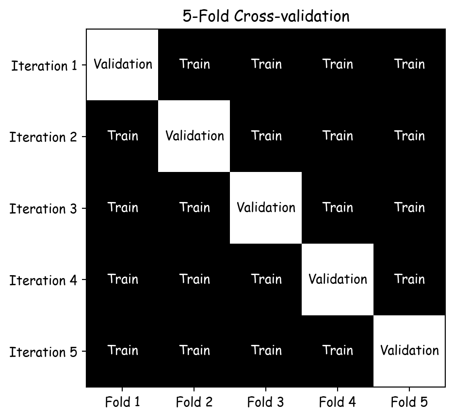
Divide the dataset into \(k\) equally sized parts (folds).
Training and validation:
- For each iteration, one fold is used as the validation set, the remaining \(k\)-1 folds are used as the training set.
Evaluation: The model’s performance is evaluated in each iteration, resulting in \(k\) performance measures.
Aggregation: Statistics are calculated based on \(k\) performance measures.

Common choices for the value of \(k\) are 3, 5, 7, and 10.

3-Fold Cross-validation

With each iteration, \(2/3\) of the dataset is used for training and \(1/3\) for validation.

Each row of the table represents an iteration within the \(k\)-fold cross-validation process, with the number of iterations equating to the number of folds. In each iteration, one fold is designated for validation, while the remaining \(k-1\) folds are utilized for training the model.

5-Fold Cross-validation

With each iteration, \(4/5\) of the dataset is used for training and \(1/5\) for validation.

More Reliable Model Evaluation

More reliable estimate of model performance compared to a single train-test split.
Reduces the variability associated with a single split, leading to a more stable and unbiased evaluation.
For large values of \(k\)¹, consider the average, variance, and confidence interval.

Better Generalization

Helps in assessing how the model generalizes to an independent dataset.
It ensures that the model’s performance is not overly optimistic or pessimistic by averaging results over multiple folds.

Efficient Use of Data

Particularly beneficial for small datasets, cross-validation ensures that every data point is used for both training and validation.
This maximizes the use of available data, leading to more accurate and reliable model training.

Some examples are more informative for learning algorithms, sometimes those near the decision boundary.

Hyperparameter Tuning

Commonly used during hyperparameter tuning, allowing for the selection of the best model parameters based on their performance across multiple folds.
This helps in identifying the optimal configuration that balances bias and variance.

Challenges

Computational Cost: Requires multiple model trainings.
- Leave-One-Out (LOO): Extreme case where ( k = N ).
Class Imbalance: Folds may not represent minority classes.
- Use Stratified Cross-Validation to maintain class proportions.
Complexity: Error-prone implementation, especially for nested cross-validation, bootstraps, or integration into larger pipelines.

Leave-one-out cross-validation (LOO-CV) can lead to overoptimistic performance evaluation, particularly in certain contexts.

Here’s why:

1.  **High Variance**: In LOO-CV, each iteration uses almost all the data for training, leaving only one instance for testing. This can result in high variance in the test error across iterations because the model is trained on nearly the full dataset. Since each training set is very similar to the full dataset, it can lead to overly optimistic estimates of generalization error, especially when the dataset is small or the model has high variance (e.g., decision trees or k-nearest neighbors).
2.  **Overfitting**: Since LOO-CV uses nearly the entire dataset for training in each iteration, complex models (especially ones prone to overfitting) can fit very closely to the data, which might result in a low training error but a misleadingly low test error in some cases.
3.  **Limited assessment of generalization**: LOO-CV might not give a reliable estimate of how well the model generalizes to completely unseen data because the difference between the training set and the full dataset is minimal, leading to a smaller gap between training and test performance.

In practice, this can make the evaluation appear more optimistic than it would be with more robust methods like k-fold cross-validation, where the test sets are larger, and the model has less opportunity to overfit the training data.

`cross_val_score`

from sklearn import tree

clf = tree.DecisionTreeClassifier()

from sklearn.model_selection import cross_val_score    

clf_scores = cross_val_score(clf, X, y, cv=5)

print("\nScores:", clf_scores)
print(f"\nMean: {clf_scores.mean():.2f}")
print(f"\nStandard deviation: {clf_scores.std():.2f}")


Scores: [0.71428571 0.66883117 0.71428571 0.79738562 0.73202614]

Mean: 0.73

Standard deviation: 0.04

sklearn.model_selection.cross_val_score, see also cross_validate.

As previously discussed, a significant limitation of decision trees is their propensity for overfitting, which leads to high variance when applied to new datasets. This issue is evident in the observed performance variability, with accuracy ranging from 67% to 79%, which is undesirable for achieving robust model generalization.

Hyperparameter tuning

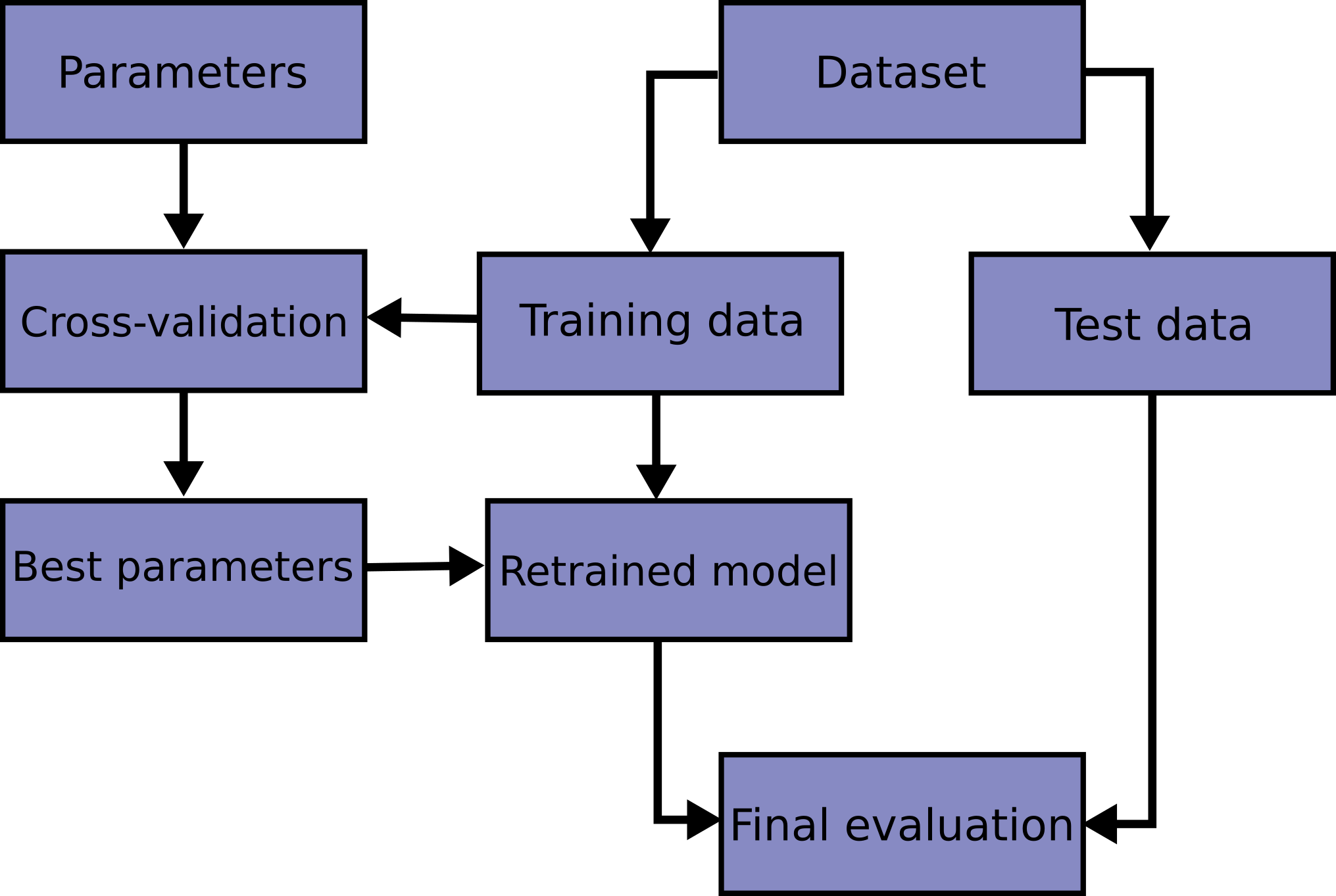
Workflow

Attribution: Cross-validation: evaluating estimator performance

The above image implicitly introduces three categories of data subsets: training, validation, and test.

Workflow - implementation

from sklearn.datasets import fetch_openml

X, y = fetch_openml(name='diabetes', version=1, return_X_y=True)

y = y.map({'tested_negative': 0, 'tested_positive': 1})

from sklearn.model_selection import train_test_split

X_train, X_test, y_train, y_test = train_test_split(X, y, test_size=0.1)

To maintain simplicity in these lecture notes, we have not applied any pre-processing steps.

Definition

A hyperparameter is a configuration external to the model that is set prior to the training process and governs the learning process, influencing model performance and complexity.

The weights of a model, which are learned by the learning algorithm, are often referred to as the model’s parameters. To avoid confusion, user-defined parameters, such as the learning rate \(\alpha\), are termed hyperparameters. Unlike model parameters, hyperparameters are not learned by the learning algorithm.

Hyperparameters - Decision Tree

criterion: gini, entropy, log_loss, measure the quality of a split.
max_depth: limits the number of levels in the tree to prevent overfitting.

See: DecisionTreeClassifier

Hyperparameters - Logistic Regression

penalty: l1 or l2, helps in preventing overfitting.
solver: liblinear, newton-cg, lbfgs, sag, saga.
max_iter: maximum number of iterations taken for the solvers to converge.
tol: stopping criteria, smaller values mean higher precision.

See: LogisticRegression and SGDClassifier.

Hyperparameters - KNN

n_neighbors: number of neighbors to use for \(k\)-neighbors queries.
weights: uniform or distance, equal weight or distance-based weight.

See: KNeighborsClassifier

Experiment: `max_depth`

for value in [3, 5, 7, None]:

  clf = tree.DecisionTreeClassifier(max_depth=value)

  clf_scores = cross_val_score(clf, X_train, y_train, cv=10)

  print("\nmax_depth = ", value)
  print(f"Mean: {clf_scores.mean():.2f}")
  print(f"Standard deviation: {clf_scores.std():.2f}")


max_depth =  3
Mean: 0.74
Standard deviation: 0.04

max_depth =  5
Mean: 0.76
Standard deviation: 0.04

max_depth =  7
Mean: 0.73
Standard deviation: 0.04

max_depth =  None
Mean: 0.71
Standard deviation: 0.05

Experiment: `criterion`

for value in ["gini", "entropy", "log_loss"]:

  clf = tree.DecisionTreeClassifier(max_depth=5, criterion=value)

  clf_scores = cross_val_score(clf, X_train, y_train, cv=10)

  print("\ncriterion = ", value)
  print(f"Mean: {clf_scores.mean():.2f}")
  print(f"Standard deviation: {clf_scores.std():.2f}")


criterion =  gini
Mean: 0.76
Standard deviation: 0.04

criterion =  entropy
Mean: 0.75
Standard deviation: 0.05

criterion =  log_loss
Mean: 0.75
Standard deviation: 0.05

For this specific problem and dataset, the criterion parameter has a limited impact on the learning process.

Experiment: `n_neighbors`

from sklearn.neighbors import KNeighborsClassifier

for value in range(1, 11):

  clf = KNeighborsClassifier(n_neighbors=value)

  clf_scores = cross_val_score(clf, X_train, y_train, cv=10)

  print("\nn_neighbors = ", value)
  print(f"Mean: {clf_scores.mean():.2f}")
  print(f"Standard deviation: {clf_scores.std():.2f}")


n_neighbors =  1
Mean: 0.67
Standard deviation: 0.05

n_neighbors =  2
Mean: 0.71
Standard deviation: 0.03

n_neighbors =  3
Mean: 0.69
Standard deviation: 0.05

n_neighbors =  4
Mean: 0.73
Standard deviation: 0.03

n_neighbors =  5
Mean: 0.72
Standard deviation: 0.03

n_neighbors =  6
Mean: 0.73
Standard deviation: 0.05

n_neighbors =  7
Mean: 0.74
Standard deviation: 0.04

n_neighbors =  8
Mean: 0.75
Standard deviation: 0.04

n_neighbors =  9
Mean: 0.73
Standard deviation: 0.05

n_neighbors =  10
Mean: 0.73
Standard deviation: 0.04

Experiment: `weights`

from sklearn.neighbors import KNeighborsClassifier

for value in ["uniform", "distance"]:

  clf = KNeighborsClassifier(n_neighbors=5, weights=value)

  clf_scores = cross_val_score(clf, X_train, y_train, cv=10)

  print("\nweights = ", value)
  print(f"Mean: {clf_scores.mean():.2f}")
  print(f"Standard deviation: {clf_scores.std():.2f}")


weights =  uniform
Mean: 0.72
Standard deviation: 0.03

weights =  distance
Mean: 0.73
Standard deviation: 0.04

For this specific problem and dataset, the weights parameter has a limited impact on the learning process.

At this point, you might hypothesize that certain combinations of hyperparameters could be more optimal than others.

Hyperparameter Tuning: Grid Search

Many hyperparameters need tuning
- Major disadvantage of ML algorithms
Manual exploration of combinations is tedious
Grid search is more systematic
1. Enumerate all possible hyperparameter combinations
2. Train on training set, evaluate on validation set

Initially, try powers of 2 or 10. Next, refine with grid search near optimal values if time permits.

The training set referred to here is different from the one previously mentioned. In each iteration of the \(k\)-fold cross-validation process, a unique training and validation set is created.

In some contexts, the choice of the model itself can be considered a hyperparameter. For instance, when performing model selection within a machine learning pipeline, different algorithms (e.g., decision trees, support vector machines, neural networks) can be treated as hyperparameters. This approach allows for the selection of the best-performing model through automated processes such as grid search or random search, alongside the tuning of other hyperparameters.

Thus, while traditionally hyperparameters refer to settings within a specific model, the model choice can also be incorporated into hyperparameter optimization frameworks.

As will be discussed later, the choice of the number of layers and the number of nodes are often considered hyperparameters when training deep learning algorithms.

`GridSearchCV`

from sklearn.model_selection import GridSearchCV

param_grid = [
  {'max_depth': range(1, 10),
   'criterion': ["gini", "entropy", "log_loss"]}
]

clf = tree.DecisionTreeClassifier()

grid_search = GridSearchCV(clf, param_grid, cv=5)

grid_search.fit(X_train, y_train)

(grid_search.best_params_, grid_search.best_score_)

({'criterion': 'gini', 'max_depth': 5}, 0.7481910124074653)

GridSearchCV

param_grid = [
  {'n_neighbors': range(1, 15),
   'weights': ["uniform", "distance"]}
]

clf = KNeighborsClassifier()

grid_search = GridSearchCV(clf, param_grid, cv=5)

grid_search.fit(X_train, y_train)

(grid_search.best_params_, grid_search.best_score_)

({'n_neighbors': 14, 'weights': 'uniform'}, 0.7554165363361485)

The variable param_grid contains a dictionary specifying the names of the parameters to be tuned, along with the respective values to be tested.

In this instance, the parameters n_neighbors and weights are being tuned. However, additional parameters could be included if necessary.

`GridSearchCV`

from sklearn.linear_model import LogisticRegression

# 2 * 5 * 5 * 3 = 150 tests!

param_grid = [
  {'penalty': ["l1", "l2", None],
   'solver' : ['liblinear', 'newton-cg', 'lbfgs', 'sag', 'saga'],
   'max_iter' : [100, 200, 400, 800, 1600],
   'tol' : [0.01, 0.001, 0.0001]}
]

clf = LogisticRegression()

grid_search = GridSearchCV(clf, param_grid, cv=5)

grid_search.fit(X_train, y_train)

(grid_search.best_params_, grid_search.best_score_)

({'max_iter': 100, 'penalty': 'l2', 'solver': 'newton-cg', 'tol': 0.001},
 0.7756646856427901)

Randomized Search

Large number of combinations (many hyperparameters, many values)
Use RandomizedSearchCV:
- Supply list of values or probability distribution for hyperparameters
- Specify number of iterations (combinations to try)
- Predictable execution time

See: Comparing randomized search and grid search for hyperparameter estimation.

Workflow

Attribution: Cross-validation: evaluating estimator performance

As the ongoing example illustrates, in addition to evaluating various hyperparameter values, multiple models can also be tested.

Finally, we proceed with testing

clf = LogisticRegression(max_iter=100, penalty='l2', solver='newton-cg', tol=0.001)

clf.fit(X_train, y_train)

y_pred = clf.predict(X_test)

from sklearn.metrics import classification_report

print(classification_report(y_test, y_pred))

              precision    recall  f1-score   support

           0       0.83      0.83      0.83        52
           1       0.64      0.64      0.64        25

    accuracy                           0.77        77
   macro avg       0.73      0.73      0.73        77
weighted avg       0.77      0.77      0.77        77

It appears that we are facing a class imbalance issue, which should have been identified earlier in our workflow!

Prologue

Summary

Training Set Size: Impact on model efficacy and generalization.
Attribute Encoding: Evaluation of techniques to capture biological phenomena.
Preprocessing:
- Data Scaling
- Handling Missing Values
- Managing Class Imbalance

Next lecture

We will further discuss machine learning engineering.

References

Russell, Stuart, and Peter Norvig. 2020. Artificial Intelligence: A Modern Approach. 4th ed. Pearson. http://aima.cs.berkeley.edu/.

Marcel Turcotte

[email protected]

School of Electrical Engineering and Computer Science (EECS)

University of Ottawa

Footnotes

10-fold cross-validation.↩︎

Preamble

Quote of the Day

Learning Objectives

Introduction

Dataset - openml

Dataset - return_X_y

Cross-evaluation

Training and test set

Common Training and Testing Ratios

Considerations for Choosing the Split Ratio

Training and test set

Training and test set

Training and test set

Definition

k-fold cross-validation

3-Fold Cross-validation

5-Fold Cross-validation

More Reliable Model Evaluation

Better Generalization

Efficient Use of Data

Hyperparameter Tuning

Challenges

cross_val_score

Hyperparameter tuning

Workflow

Workflow - implementation

Definition

Hyperparameters - Decision Tree

Hyperparameters - Logistic Regression

Hyperparameters - KNN

Experiment: max_depth

Experiment: criterion

Experiment: n_neighbors

Experiment: weights

Hyperparameter Tuning: Grid Search

GridSearchCV

GridSearchCV

GridSearchCV

Randomized Search

Workflow

Finally, we proceed with testing

Prologue

Summary

Next lecture

References

Footnotes

Dataset - `return_X_y`

`cross_val_score`

Experiment: `max_depth`

Experiment: `criterion`

Experiment: `n_neighbors`

Experiment: `weights`

`GridSearchCV`

`GridSearchCV`